The ordinary least squares estimator of the coefficient of a first-order autoregressive process is consistent and asymptotically normal, but it is biased in finite samples: on average, it underestimates the persistence of the process. This note explains where the bias comes from, namely the fact that the regressor is not strictly exogenous, derives the classical approximation \(-2\rho/T\) by a first-order expansion, and then confronts it with Monte Carlo simulations in Python: bias as a function of the sample size and of the persistence, distribution of the estimator, and two ways of correcting the bias, analytical and by bootstrap. The solutions to the exercises are given in collapsible blocks.
The model and the estimator
Consider a first-order autoregressive process:
\begin{equation*} y_t = \rho\,y_{t-1} + \varepsilon_t,\qquad t = 1,\dots,T \end{equation*}where \(|\rho| < 1\) and the innovations \(\varepsilon_t\) are independent and identically distributed according to a normal distribution with mean zero and variance \(\sigma^2\). We assume that the process starts at \(y_0 = 0\), so that \(y_1 = \varepsilon_1\). The process is then not stationary but asymptotically stationary: the variance of \(y_t\), \(\sigma^2(1-\rho^{2t})/(1-\rho^2)\), converges to the stationary variance \(\gamma_0 = \sigma^2/(1-\rho^2)\). We shall see in an exercise that this choice of initial condition has practically no effect on the results.
We observe a sample \(y_1,\dots,y_T\) and wish to estimate \(\rho\). The ordinary least squares (OLS) estimator, obtained by regressing \(y_t\) on \(y_{t-1}\) without an intercept, is:
\begin{equation*} \hat\rho = \frac{\sum_{t=2}^T y_t\,y_{t-1}}{\sum_{t=2}^T y_{t-1}^2} \end{equation*}It is also the maximum likelihood estimator conditional on the first observation, since the conditional log-likelihood is, up to a constant, \(-\frac{1}{2\sigma^2}\sum_{t=2}^T(y_t - \rho y_{t-1})^2\), which \(\hat\rho\) maximises. Substituting \(y_t = \rho y_{t-1} + \varepsilon_t\) in the numerator yields the decomposition that will be used throughout:
\begin{equation*} \hat\rho - \rho = \frac{\sum_{t=2}^T y_{t-1}\,\varepsilon_t}{\sum_{t=2}^T y_{t-1}^2} \equiv \frac{N}{D} \end{equation*}The estimation error is the ratio of two random variables, a numerator \(N\) and a denominator \(D\), both of which depend on the innovations.
Show that the distribution of \(\hat\rho\) does not depend on \(\sigma^2\). The bias of the estimator is therefore a function of \(\rho\) and \(T\) only.
Solution
Write \(\varepsilon_t = \sigma\eta_t\), where the \(\eta_t\) are independent standard normal variables. By induction from \(y_0 = 0\), \(y_t = \sigma\sum_{j=0}^{t-1}\rho^j\eta_{t-j} \equiv \sigma z_t\), where the process \(z_t\) depends only on \(\rho\) and on the \(\eta_t\). Substituting into the estimator:
\begin{equation*} \hat\rho = \frac{\sigma^2\sum_{t=2}^T z_t\,z_{t-1}}{\sigma^2\sum_{t=2}^T z_{t-1}^2} = \frac{\sum_{t=2}^T z_t\,z_{t-1}}{\sum_{t=2}^T z_{t-1}^2} \end{equation*}The factor \(\sigma^2\) cancels: \(\hat\rho\) is a function of \(\rho\), \(T\) and the \(\eta_t\) only, and so is its distribution. In the simulations we may therefore set \(\sigma = 1\) without loss of generality.
Consistency and asymptotic distribution
The OLS estimator is consistent and asymptotically normal:
\begin{equation*} \hat\rho \xrightarrow[T\to\infty]{p} \rho \qquad\text{and}\qquad \sqrt T\,(\hat\rho - \rho) \xrightarrow[T\to\infty]{d} \mathcal N\bigl(0, 1-\rho^2\bigr) \end{equation*}Divide the numerator and the denominator of \(\hat\rho - \rho\) by \(T\). The process \(y_t\) being asymptotically stationary and ergodic, the law of large numbers gives \(\frac1T\sum_{t=2}^Ty_{t-1}^2 \to \gamma_0 = \sigma^2/(1-\rho^2)\) in probability. The term \(y_{t-1}\varepsilon_t\) has mean zero, since \(\varepsilon_t\) is independent of \(y_{t-1}\), which depends only on past innovations, and \(\mathbb E[\varepsilon_t] = 0\); moreover the terms \(y_{t-1}\varepsilon_t\) are uncorrelated, since for \(s < t\) we have \(\mathbb E[y_{s-1}\varepsilon_sy_{t-1}\varepsilon_t] = \mathbb E[y_{s-1}\varepsilon_sy_{t-1}]\,\mathbb E[\varepsilon_t] = 0\). The law of large numbers therefore gives \(\frac1T\sum_{t=2}^Ty_{t-1}\varepsilon_t \to 0\), whence the convergence of \(\hat\rho\) to \(\rho\). For the asymptotic distribution, we take for granted that the central limit theorem applies to the sequence \(y_{t-1}\varepsilon_t\), whose terms have mean zero, are uncorrelated and have variance \(\mathbb E[y_{t-1}^2]\,\mathbb E[\varepsilon_t^2] \to \gamma_0\sigma^2\)1:
\begin{equation*} \frac{1}{\sqrt T}\sum_{t=2}^Ty_{t-1}\varepsilon_t \xrightarrow{d} \mathcal N\bigl(0, \gamma_0\sigma^2\bigr) \end{equation*}By Slutsky's theorem, \(\sqrt T(\hat\rho - \rho)\) converges in distribution to a centred normal with variance \(\gamma_0\sigma^2/\gamma_0^2 = \sigma^2/\gamma_0 = 1-\rho^2\).
The asymptotic variance \(1-\rho^2\) does not depend on \(\sigma^2\), in line with the previous exercise, and it decreases as persistence increases: the closer \(\rho\) is to one, the more dispersed the regressor \(y_{t-1}\) is relative to the innovation, and the more precise the estimator. In large samples, the distribution of \(\hat\rho\) is therefore approximated by \(\mathcal N\bigl(\rho, (1-\rho^2)/T\bigr)\), a distribution centred on the true value. This approximation says nothing about the finite-sample bias, which is of order \(1/T\) and disappears in the normalisation by \(\sqrt T\).
A finite-sample bias
In the linear regression model with deterministic regressors, the OLS estimator is unbiased because the expectation of the error is zero conditional on all the regressors. Here the regressor is random, and while \(\mathbb E[\varepsilon_t\mid y_{t-1}] = 0\) does hold, \(\mathbb E[\varepsilon_t\mid y_1,\dots,y_{T-1}] = 0\) does not: the innovation \(\varepsilon_t\) enters \(y_t\), \(y_{t+1}\), …, which are the regressors of the following dates. The regressor is predetermined, not strictly exogenous. To see how this dependence produces a bias, write the estimation error as a weighted sum of the innovations:
\begin{equation*} \hat\rho - \rho = \sum_{t=2}^T w_t\,\varepsilon_t \qquad\text{with}\qquad w_t = \frac{y_{t-1}}{\sum_{s=2}^Ty_{s-1}^2} \end{equation*}If the weights \(w_t\) were independent of the innovations, each term would have zero expectation. But the weight \(w_t\) depends on \(\varepsilon_t\) through its denominator: a positive innovation raises \(y_t\), \(y_{t+1}\), …, hence the denominator, and lowers the weight given to that innovation. A positive innovation thus receives, on average, a smaller weight than a negative innovation of the same size, and the weighted sum is negative in expectation when \(\rho > 0\). The following property quantifies this effect.
To first order in \(1/T\), the bias of the OLS estimator is2:
\begin{equation*} \mathbb E[\hat\rho] - \rho = -\frac{2\rho}{T} + O\!\left(\frac{1}{T^2}\right) \end{equation*}We give the derivation by a first-order expansion, whose validity we take for granted3. Write \(\bar D = \mathbb E[D]\) and \(D = \bar D(1 + \delta)\) with \(\delta = (D-\bar D)/\bar D\), which is of order \(1/\sqrt T\). The expansion \((1+\delta)^{-1} = 1 - \delta + O(\delta^2)\) gives:
\begin{equation*} \begin{split} \hat\rho - \rho &= \frac{N}{\bar D}(1 - \delta) + \dots\\ \mathbb E[\hat\rho] - \rho &= \frac{\mathbb E[N]}{\bar D} - \frac{\mathbb E[N D]}{\bar D^2} + \dots = -\frac{\mathbb E[ND]}{\bar D^2} + \dots \end{split} \end{equation*}since \(\mathbb E[N] = 0\) and \(\mathbb E[N\bar D] = 0\). It remains to compute \(\mathbb E[ND] = \sum_{t=2}^T\sum_{s=2}^T\mathbb E\bigl[y_{t-1}\varepsilon_t\,y_{s-1}^2\bigr]\). If \(s\leq t\), \(y_{s-1}\) depends only on innovations prior to \(\varepsilon_t\) and the term vanishes. If \(s > t\), we isolate in \(y_{s-1}\) the contribution of \(y_{t-1}\) and of \(\varepsilon_t\):
\begin{equation*} y_{s-1} = \rho^{s-t}y_{t-1} + \rho^{s-t-1}\varepsilon_t + u_{s,t} \qquad\text{with}\qquad u_{s,t} = \sum_{j=t+1}^{s-1}\rho^{s-1-j}\varepsilon_j \end{equation*}where \(u_{s,t}\) has mean zero and is independent of \((y_{t-1},\varepsilon_t)\). Expanding the square \(y_{s-1}^2\) and multiplying by \(y_{t-1}\varepsilon_t\), all terms have zero expectation (they contain \(\varepsilon_t\) or \(u_{s,t}\) to an odd power, or \(y_{t-1}\) to an odd power with \(\varepsilon_t\) to an even power), except the cross product:
\begin{equation*} \mathbb E\bigl[y_{t-1}\varepsilon_t\,y_{s-1}^2\bigr] = 2\rho^{2(s-t)-1}\,\mathbb E\bigl[y_{t-1}^2\bigr]\,\mathbb E\bigl[\varepsilon_t^2\bigr] = 2\rho^{2(s-t)-1}\sigma^2\,\mathbb E\bigl[y_{t-1}^2\bigr] \end{equation*}Summing over \(s = t+1,\dots,T\) gives the geometric series \(\rho(1-\rho^{2(T-t)})/(1-\rho^2)\). To leading order, we may replace \(\mathbb E[y_{t-1}^2]\) by the stationary variance \(\gamma_0\) and the geometric sum by its limit \(\rho/(1-\rho^2)\), the discrepancies affecting only a bounded number of terms at the edges of the sample, which only changes the terms of order \(1/T^2\) of the bias:
\begin{equation*} \mathbb E[ND] \simeq (T-1)\,\frac{2\rho\sigma^2\gamma_0}{1-\rho^2} = 2\rho\,(T-1)\,\gamma_0^2 \qquad\text{and}\qquad \bar D \simeq (T-1)\,\gamma_0 \end{equation*}where we used \(\sigma^2/(1-\rho^2) = \gamma_0\). Finally:
\begin{equation*} \mathbb E[\hat\rho] - \rho \simeq -\frac{2\rho\,(T-1)\,\gamma_0^2}{(T-1)^2\gamma_0^2} = -\frac{2\rho}{T-1} = -\frac{2\rho}{T} + O\!\left(\frac{1}{T^2}\right) \end{equation*}The bias is negative for \(\rho > 0\), proportional to \(\rho\) and inversely proportional to the sample size. It vanishes to first order when \(\rho = 0\). It does not depend on \(\sigma^2\), in line with the exercise of the first section. For a sample of \(50\) observations and \(\rho = 0.9\), the approximation gives a bias of \(-0.036\), which is not negligible: the half-life of a shock, \(\log(1/2)/\log\rho\), falls from \(6.6\) periods with \(\rho = 0.9\) to \(4.7\) periods with \(\rho = 0.864\).
When the regression includes an intercept, that is, when the mean of the process is estimated along with \(\rho\), the bias is larger. Kendall (Biometrika, 1954) showed that to first order it equals \(-(1+3\rho)/T\). Even under the hypothesis \(\rho = 0\), the first-order sample autocorrelation is therefore biased downwards, by \(-1/T\). This case is treated in an exercise at the end of the note.
Monte Carlo simulations
To measure the bias we proceed by simulation. We draw \(B\) samples of
size \(T\) from the process, compute the estimator on each of them, and the
mean of the \(B\) estimates, minus the true value, approximates the bias
with an error of order \(1/\sqrt B\). The following function simulates \(B\)
trajectories at once: each row of the array y is a sample, and the loop
only runs over time.
rng = np.random.default_rng(2014)

def simulate_ar1(T, rho, B, sigma=1.0):
    epsilon = sigma*rng.standard_normal((B, T))
    y = np.zeros((B, T+1))
    for t in range(1, T+1):
        y[:, t] = rho*y[:, t-1] + epsilon[:, t-1]
    return y[:, 1:]

def estimate_ar1(y):
    return (y[:, 1:]*y[:, :-1]).sum(axis=1)/(y[:, :-1]**2).sum(axis=1)
We start with \(\rho = 0.9\) and sample sizes from \(10\) to \(460\), with \(B = 20\,000\) replications.
B = 20000
rho0 = 0.9
for T in range(10, 501, 50):
    bias = estimate_ar1(simulate_ar1(T, rho0, B)).mean() - rho0
    print(T, round(bias, 4), round(-2*rho0/T, 4))
| \(T\) | Simulated bias | \(-2\rho/T\) |
|---|---|---|
| 10 | \(-0.134\) | \(-0.180\) |
| 60 | \(-0.028\) | \(-0.030\) |
| 110 | \(-0.016\) | \(-0.016\) |
| 160 | \(-0.011\) | \(-0.011\) |
| 210 | \(-0.008\) | \(-0.009\) |
| 260 | \(-0.007\) | \(-0.007\) |
| 310 | \(-0.006\) | \(-0.006\) |
| 360 | \(-0.005\) | \(-0.005\) |
| 410 | \(-0.004\) | \(-0.004\) |
| 460 | \(-0.004\) | \(-0.004\) |
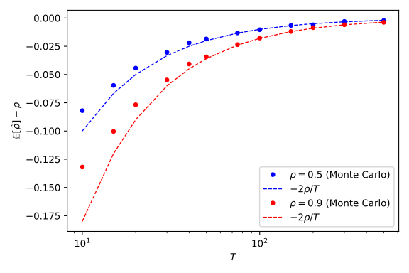
The first-order approximation is excellent as soon as the sample has about sixty observations. For very small samples it overstates the bias: with \(T = 10\), the simulated bias is \(-0.134\) against a predicted \(-0.180\), the terms of order \(1/T^2\) no longer being negligible. The figure below repeats this comparison for two values of \(\rho\).
Effect of persistence
For a given sample size, the bias grows with \(\rho\), linearly according to the approximation. To plot the bias as a function of \(\rho\) without the simulation noise blurring the curve, we use the same innovations for all values of \(\rho\): the estimates obtained for two neighbouring values of \(\rho\) are then strongly correlated, and their difference is measured much more precisely than each of them.
def simulate_ar1_with(epsilon, rho):
    B, T = epsilon.shape
    y = np.zeros((B, T+1))
    for t in range(1, T+1):
        y[:, t] = rho*y[:, t-1] + epsilon[:, t-1]
    return y[:, 1:]

rho_grid = np.linspace(0, 0.98, 50)
bias_rho = {}
for T in (25, 50, 100):
    epsilon = rng.standard_normal((B, T))
    bias_rho[T] = [estimate_ar1(simulate_ar1_with(epsilon, rho)).mean() - rho for rho in rho_grid]
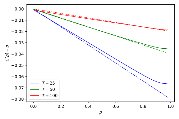
The figure above confirms the proportionality to \(\rho\) for moderate values of the persistence, and shows that the approximation deteriorates as \(\rho\) approaches one, especially in small samples: the simulated bias bends and remains smaller in absolute value than \(2\rho/T\). In the vicinity of the unit root, the distribution of the estimator changes nature and the expansion in powers of \(1/T\) is no longer adequate.
Distribution of the estimator
The bias is only one aspect of the finite-sample distribution of \(\hat\rho\). The figure below compares the density of the estimator, estimated by a kernel method from the \(B\) replications, with the asymptotic approximation \(\mathcal N\bigl(\rho, (1-\rho^2)/T\bigr)\).
fig, axes = plt.subplots(1, 3, figsize=(12, 4))
x = np.linspace(-0.6, 1.2, 600)
for ax, rho in zip(axes, (0.0, 0.5, 0.9)):
    for T, c in ((25, 'b'), (100, 'r')):
        rhohat = estimate_ar1(simulate_ar1(T, rho, B))
        ax.plot(x, gaussian_kde(rhohat)(x), c, linewidth=1, label=fr'$T = {T}$')
        ax.plot(x, norm.pdf(x, rho, np.sqrt((1-rho**2)/T)), c+':', linewidth=1,
                label=fr'$\mathcal{{N}}(\rho, (1-\rho^2)/{T})$')
    ax.axvline(rho, color='k', linewidth=0.5)
    ax.set_xlim(rho-0.7, min(rho+0.7, 1.15))
    ax.set_xlabel(r'$\hat\rho$'); ax.set_title(fr'$\rho = {rho}$')
    ax.legend(fontsize=8)
fig.tight_layout()
fig.savefig("ar1-densites.svg", transparent=True)
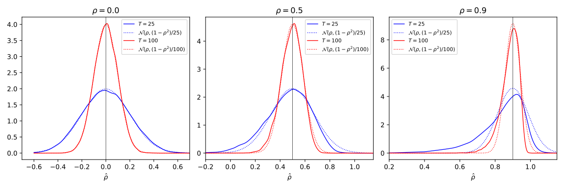
For \(\rho = 0\) the asymptotic distribution is a good approximation even with \(25\) observations. For \(\rho = 0.5\) the distribution is shifted to the left, which is the bias, and slightly asymmetric. For \(\rho = 0.9\) the asymmetry becomes pronounced: the distribution has a long left tail and is compressed on the right, the estimator rarely exceeding one. The normal distribution, symmetric around \(\rho\), then poorly describes the uncertainty about the estimate, and a confidence interval built on the asymptotic distribution is too optimistic on the low-persistence side.
Correcting the bias
Since \(\mathbb E[\hat\rho] \simeq \rho(1-2/T)\), a corrected estimator follows immediately:
\begin{equation*} \tilde\rho = \frac{T}{T-2}\,\hat\rho \end{equation*}whose expectation is \(\rho + O(1/T^2)\). This analytical correction has a cost: the variance of \(\tilde\rho\) is that of \(\hat\rho\) multiplied by \((T/(T-2))^2\). In small samples, where the correction is useful, this inflation is not negligible, and the gain must be measured in mean squared error.
A second approach, which does not assume the form of the bias to be known, is the parametric bootstrap. From a sample we compute \(\hat\rho\), we simulate \(R\) artificial samples of the process \(y_t = \hat\rho\,y_{t-1} + \varepsilon_t\), we re-estimate \(\rho\) on each of them, and the mean of the \(R\) estimates \(\hat\rho^{\star}_r\), minus \(\hat\rho\), estimates the bias. The bootstrap bias-corrected estimator is:
\begin{equation*} \hat\rho_{\text{boot}} = \hat\rho - \Bigl(\frac1R\sum_{r=1}^R\hat\rho^{\star}_r - \hat\rho\Bigr) = 2\hat\rho - \frac1R\sum_{r=1}^R\hat\rho^{\star}_r \end{equation*}The bias is thus evaluated at \(\hat\rho\) rather than at \(\rho\), which introduces an error of order \(1/T^2\) only, the bias function being smooth. The following function applies the correction to \(B\) samples simultaneously, nesting the \(R\) bootstrap replications in an additional dimension.
def bootstrap(y, R=199):
    B, T = y.shape
    rhohat = estimate_ar1(y)
    rhostar = np.empty((B, R))
    for r in range(R):
        z = simulate_ar1_with(rng.standard_normal((B, T)), rhohat)
        rhostar[:, r] = estimate_ar1(z)
    return 2*rhohat - rhostar.mean(axis=1)

for T in (25, 50, 100):
    y = simulate_ar1(T, rho0, B)
    estimators = {'OLS': estimate_ar1(y), 'corrected': T*estimate_ar1(y)/(T-2), 'bootstrap': bootstrap(y)}
    for name, e in estimators.items():
        print(T, name, round(e.mean() - rho0, 4), round(e.std(), 4), round(np.sqrt(((e - rho0)**2).mean()), 4))
The following table reports, for \(\rho = 0.9\), the bias, the standard deviation and the root mean squared error (RMSE) of the three estimators.
| \(T\) | Estimator | Bias | Std. dev. | RMSE |
|---|---|---|---|---|
| 25 | OLS | \(-0.065\) | \(0.134\) | \(0.149\) |
| 25 | Corrected | \(+0.007\) | \(0.146\) | \(0.146\) |
| 25 | Bootstrap | \(-0.006\) | \(0.142\) | \(0.142\) |
| 50 | OLS | \(-0.034\) | \(0.080\) | \(0.087\) |
| 50 | Corrected | \(+0.002\) | \(0.083\) | \(0.083\) |
| 50 | Bootstrap | \(-0.001\) | \(0.083\) | \(0.083\) |
| 100 | OLS | \(-0.018\) | \(0.051\) | \(0.054\) |
| 100 | Corrected | \(+0.000\) | \(0.052\) | \(0.052\) |
| 100 | Bootstrap | \(-0.001\) | \(0.052\) | \(0.052\) |
Both corrections remove most of the bias, at the price of a modest increase in the standard deviation, and reduce the mean squared error. The bootstrap does slightly better than the analytical correction in the smallest sample, where the approximation \(-2\rho/T\) overstates the bias, as we saw; the two methods are equivalent beyond \(50\) observations. The analytical correction has the advantage of being immediate, the bootstrap that of extending without further calculation to models for which no formula is available.
Beyond the AR(1)
The mechanism behind the bias owes nothing to the dimension of the model or to the order of the process: as soon as the regressors contain lagged values of the dependent variable, they are predetermined without being strictly exogenous, and the OLS or maximum likelihood estimator is biased to order \(1/T\). What changes with the model is the possibility of writing the bias explicitly, and the form taken by the small-sample difficulties.
AR(p) processes
For an autoregressive process of order \(p\), the first-order expansion proceeds in the same way, with matrices in place of scalars, and the bias of each coefficient is a linear combination of the coefficients, divided by \(T\). The explicit formulas are due to Tjøstheim and Paulsen (Biometrika, 1983) and, for the regression with an intercept, to Shaman and Stine (Journal of the American Statistical Association, 1988). The qualitative result is that of the AR(1): persistence is underestimated, the sum of the autoregressive coefficients, which governs the half-life of shocks, being biased downwards by an amount comparable to \(-(1+3\rho)/T\) where \(\rho\) would be the sum of the coefficients. The two corrections of the previous section apply unchanged, the analytical formula only requiring the bias to be evaluated at the estimated point.
VAR(p) processes
The vector case is the one where bias correction matters most in practice, since VAR models are estimated on short samples, with many parameters, and are used to compute impulse response functions that depend non-linearly on the coefficients. For a VAR(1) in \(n\) variables, \(Y_t = c + A\,Y_{t-1} + \varepsilon_t\), where \(\varepsilon_t\) is a white noise with variance matrix \(\Sigma\), Nicholls and Pope (Australian Journal of Statistics, 1988) generalised Kendall's formula:
\begin{equation*} \begin{split} \mathbb E[\hat A] - A &\simeq -\frac{1}{T}\,\Sigma\,M\,\Gamma_0^{-1}\\ M &= (I_n - A^\top)^{-1} + A^\top(I_n - A^{\top 2})^{-1} + \sum_{k=1}^n\lambda_k\,(I_n - \lambda_kA^\top)^{-1} \end{split} \end{equation*}where the \(\lambda_k\) are the eigenvalues of \(A\) and \(\Gamma_0\) the stationary variance matrix of \(Y_t\), the solution of \(\Gamma_0 = A\,\Gamma_0A^\top + \Sigma\). For \(n = 1\), with \(\Sigma = \sigma^2\), \(\Gamma_0 = \sigma^2/(1-\rho^2)\) and \(\lambda_1 = \rho\), the matrix \(M\) equals \((1-\rho)^{-1} + 2\rho(1-\rho^2)^{-1}\) and we recover \(-(1+3\rho)/T\); without an intercept, the first term of \(M\), which comes from the estimation of the mean, disappears, and \(-2\rho/T\) remains. A VAR(p) reduces to a VAR(1) through its companion representation, and the formula applies to the companion matrix, as shown by Pope (Journal of Time Series Analysis, 1990). Kilian (Review of Economics and Statistics, 1998) proposed to correct the bias of the coefficients, by this formula or by bootstrap, before computing impulse responses and their confidence intervals: the downward bias in persistence translates into responses that die out too quickly, and intervals built without correction are shifted. An exercise proposes to check the formula on a bivariate VAR.
ARMA(p,q) processes
When the model has a moving average part, the maximum likelihood estimator, exact or conditional, no longer has an explicit form, and neither does its finite-sample bias. The simulations of Ansley and Newbold (Journal of Econometrics, 1980) show biases of the same order as for autoregressive processes, with an additional difficulty specific to moving average coefficients: the likelihood reaches its maximum on the invertibility boundary, \(\hat\theta = \pm1\), with strictly positive probability, even when the true coefficient is well inside: for an MA(1) with \(\theta = 0.8\) and \(T = 50\), Cryer and Ledolter (Biometrika, 1981) put it at \(0.13\). This pile-up of the distribution of the estimator on the boundary, studied by Sargan and Bhargava (Econometrica, 1983), makes the distribution of \(\hat\theta\) bimodal, with a point mass at one, and no proportional correction can recentre it. The parametric bootstrap remains usable to estimate the bias, provided the model is re-estimated on each artificial sample, which has a numerical cost, and the invertible solution is retained.
State-space models
The parameters of a state-space model are estimated by maximum likelihood, the likelihood being computed by the Kalman filter from the prediction errors. Nothing new as far as the bias is concerned, since ARMA models are a special case, but the pile-up phenomenon takes a form worth knowing. In the local level model, \(y_t = \mu_t + \varepsilon_t\) and \(\mu_t = \mu_{t-1} + \eta_t\), the maximum likelihood estimator of the variance of \(\eta_t\) is exactly zero with strictly positive probability, even if this variance is positive (Shephard and Harvey, Journal of Time Series Analysis, 1990). The level is then estimated as constant, and the model reduces to a white noise around a mean. This is no coincidence: the local level model is equivalent to an ARIMA(0,1,1), and a zero variance of \(\eta_t\) corresponds to \(\theta = -1\), the invertibility boundary. For this kind of parameter, Stock and Watson (Journal of the American Statistical Association, 1998) proposed a median-unbiased estimator, obtained by inverting a function of the test statistic for constancy of the level, computed by simulation. The bootstrap of state-space models, which resamples the standardised innovations of the Kalman filter, was developed by Stoffer and Wall (Journal of the American Statistical Association, 1991).
Correcting the expectation is not the only way to recentre an estimator. Andrews (Econometrica, 1993) built for the AR(1) a median-unbiased estimator: one computes, by simulation, the median of \(\hat\rho\) for each value of \(\rho\), and inverts this function at the observed \(\hat\rho\). This construction remains valid in the vicinity of the unit root, where the expansion in powers of \(1/T\) is no longer adequate and the distribution of the estimator is very asymmetric, as we saw on the figure of the densities. It extends to models with an intercept and a trend, and it is the one Stock and Watson take up for the variances of state-space models.
Exercises
We now estimate \(\rho\) by OLS in a regression with an intercept, \(y_t = c + \rho\,y_{t-1} + \varepsilon_t\). Write down the estimator of \(\rho\), simulate its bias for \(\rho = 0\), \(0.5\) and \(0.9\) and \(T = 25\), \(50\), \(100\), and compare with Kendall's approximation, \(-(1+3\rho)/T\).
Solution
In the regression with an intercept, the estimator of \(\rho\) is the coefficient of the regression of \(y_t\) on \(y_{t-1}\) after centring both variables on their sample means (computed over \(t = 2,\dots,T\) for \(y_t\) and over \(t = 1,\dots,T-1\) for \(y_{t-1}\)):
\begin{equation*} \hat\rho_c = \frac{\sum_{t=2}^T(y_t - \bar y_{(1)})(y_{t-1} - \bar y_{(0)})}{\sum_{t=2}^T(y_{t-1} - \bar y_{(0)})^2} \end{equation*}def estimate_ar1_intercept(y):
y1 = y[:, 1:] - y[:, 1:].mean(axis=1, keepdims=True)
y0 = y[:, :-1] - y[:, :-1].mean(axis=1, keepdims=True)
return (y1*y0).sum(axis=1)/(y0**2).sum(axis=1)
for rho in (0.0, 0.5, 0.9):
for T in (25, 50, 100):
bias = estimate_ar1_intercept(simulate_ar1(T, rho, B)).mean() - rho
print(rho, T, round(bias, 4), round(-(1+3*rho)/T, 4))
| \(\rho\) | \(T\) | Simulated bias | \(-(1+3\rho)/T\) |
|---|---|---|---|
| \(0\) | 25 | \(-0.041\) | \(-0.040\) |
| \(0\) | 50 | \(-0.019\) | \(-0.020\) |
| \(0\) | 100 | \(-0.010\) | \(-0.010\) |
| \(0.5\) | 25 | \(-0.103\) | \(-0.100\) |
| \(0.5\) | 50 | \(-0.053\) | \(-0.050\) |
| \(0.5\) | 100 | \(-0.024\) | \(-0.025\) |
| \(0.9\) | 25 | \(-0.182\) | \(-0.148\) |
| \(0.9\) | 50 | \(-0.087\) | \(-0.074\) |
| \(0.9\) | 100 | \(-0.041\) | \(-0.037\) |
The bias is markedly larger than without an intercept, and it no longer vanishes when \(\rho = 0\): centring introduces a negative correlation between the deviations from the mean of \(y_t\) and of \(y_{t-1}\), even for a white noise. Kendall's approximation is good for moderate persistence, but understates the bias when \(\rho = 0.9\), especially in small samples, contrary to what we observed without an intercept.
The simulations start at \(y_0 = 0\). Redo the computation of the bias of \(\hat\rho\) for \(\rho = 0.9\) and \(T = 25\), \(50\), \(100\), drawing the initial condition from the stationary distribution, \(y_0\sim\mathcal N(0, \gamma_0)\), and compare.
Solution
It suffices to initialise the first column of the array with draws of standard deviation \(\sqrt{\gamma_0} = \sigma/\sqrt{1-\rho^2}\).
def simulate_ar1_stationary(T, rho, B, sigma=1.0):
    epsilon = sigma*rng.standard_normal((B, T))
    y = np.zeros((B, T+1))
    y[:, 0] = sigma/np.sqrt(1-rho**2)*rng.standard_normal(B)
    for t in range(1, T+1):
        y[:, t] = rho*y[:, t-1] + epsilon[:, t-1]
    return y[:, 1:]

for T in (25, 50, 100):
    b0 = estimate_ar1(simulate_ar1(T, rho0, B)).mean() - rho0
    b1 = estimate_ar1(simulate_ar1_stationary(T, rho0, B)).mean() - rho0
    print(T, round(b0, 4), round(b1, 4))
| \(T\) | \(y_0 = 0\) | Stationary \(y_0\) |
|---|---|---|
| 25 | \(-0.065\) | \(-0.058\) |
| 50 | \(-0.034\) | \(-0.032\) |
| 100 | \(-0.017\) | \(-0.017\) |
Starting from the stationary distribution slightly reduces the bias, by a little less than one hundredth for \(T = 25\), by two thousandths for \(T = 50\), and the difference is no longer measurable for \(T = 100\), the simulation error being about \(0.001\) with \(20\,000\) replications. The difference is divided by four each time \(T\) doubles, which is indeed the behaviour of a \(1/T^2\) term. With \(\rho = 0.9\) the process nevertheless takes several dozen periods to reach its stationary variance, but the initial condition only affects the first terms of the sums, whose weight is of order \(1/T\), hence an effect of order \(1/T^2\) on the bias, in line with the proof of the property.
Check by simulation the Nicholls and Pope formula for the bivariate VAR(1) with intercept defined by:
\begin{equation*} A = \begin{pmatrix} 0.6 & 0.2\\ -0.1 & 0.8\end{pmatrix} \qquad\text{and}\qquad \Sigma = \begin{pmatrix} 1 & 0.3\\ 0.3 & 1\end{pmatrix} \end{equation*}for \(T = 50\), \(100\) and \(200\).
Solution
The OLS estimator of \(A\) is \(\hat A = \bigl(\sum_tY_tY_{t-1}^\top\bigr)\bigl(\sum_tY_{t-1}Y_{t-1}^\top\bigr)^{-1}\),
the variables being centred on their sample means since the regression
includes an intercept. The matrix \(\Gamma_0\) is obtained by solving the
discrete Lyapunov equation, which solve_discrete_lyapunov from scipy
does.
from scipy.linalg import solve_discrete_lyapunov

A = np.array([[0.6, 0.2], [-0.1, 0.8]])
Sigma = np.array([[1.0, 0.3], [0.3, 1.0]])
n = 2

def simulate_var1(T, B):
    epsilon = rng.standard_normal((B, T, n)) @ np.linalg.cholesky(Sigma).T
    y = np.zeros((B, T+1, n))
    for t in range(1, T+1):
        y[:, t] = y[:, t-1] @ A.T + epsilon[:, t-1]
    return y[:, 1:]

def estimate_var1(y):
    y1 = y[:, 1:] - y[:, 1:].mean(axis=1, keepdims=True)
    y0 = y[:, :-1] - y[:, :-1].mean(axis=1, keepdims=True)
    S10 = np.einsum('bti,btj->bij', y1, y0)
    S00 = np.einsum('bti,btj->bij', y0, y0)
    return S10 @ np.linalg.inv(S00)

Gamma0 = solve_discrete_lyapunov(A, Sigma)
I, At = np.eye(n), A.T
bracket = np.linalg.inv(I - At) + At @ np.linalg.inv(I - At @ At)
bracket = bracket + sum(lam*np.linalg.inv(I - lam*At) for lam in np.linalg.eigvals(A))
bias_pope = -(Sigma @ bracket @ np.linalg.inv(Gamma0)).real

for T in (50, 100, 200):
    bias_mc = estimate_var1(simulate_var1(T, B)).mean(axis=0) - A
    print(T, np.round(bias_mc, 3).tolist(), np.round(bias_pope/T, 3).tolist())
| \(T\) | Simulated bias | Nicholls and Pope |
|---|---|---|
| 50 | \(\begin{pmatrix} -0.073 & 0.022\\ -0.019 & -0.067\end{pmatrix}\) | \(\begin{pmatrix} -0.070 & 0.024\\ -0.020 & -0.059\end{pmatrix}\) |
| 100 | \(\begin{pmatrix} -0.036 & 0.011\\ -0.009 & -0.033\end{pmatrix}\) | \(\begin{pmatrix} -0.035 & 0.012\\ -0.010 & -0.030\end{pmatrix}\) |
| 200 | \(\begin{pmatrix} -0.018 & 0.006\\ -0.005 & -0.015\end{pmatrix}\) | \(\begin{pmatrix} -0.017 & 0.006\\ -0.005 & -0.015\end{pmatrix}\) |
The agreement is good from \(T = 100\) onwards, and the order of magnitude is the same as for the AR(1): the two diagonal coefficients, which carry the persistence of each variable, are biased downwards by about \(-0.07\) for \(T = 50\), a tenth of their value. The bias of the cross coefficient \(a_{1,2}\) is positive: in the vector case, the bias of a coefficient depends on the whole matrix \(A\), and its sign is not necessarily opposite to that of the coefficient.
Footnotes:
The sequence \(y_{t-1}\varepsilon_t\) is a martingale difference, and the central limit theorem for martingale differences applies.
This result is due to Marriott and Pope (Biometrika, 1954) and White (Biometrika, 1961); the bias of the OLS estimator in dynamic models was first pointed out by Hurwicz (1950), in the Cowles Commission volume edited by Koopmans, and it is sometimes called the Hurwicz bias.
The rigorous justification of the expansion, and the computation of the higher-order terms, are in White's (1961) article.