The note on country-specific convergence speeds ended on a doubt: the Solow model was rejected there, but a simulation showed that this rejection could come from the endogeneity of initial income, which a cross-section cannot remove. A panel can, by letting each country have its own level of labour efficiency. It comes at a higher price than advertised: the most usual estimator, the within estimator, barely responds to the parameter it is meant to measure, and this has to be shown by simulation before it is believed. This note introduces panel data for readers who have never used them, estimates the model, measures the bias, and corrects it by indirect inference, a method explained step by step. It then answers the questions of the previous note. The estimates of the speed — 0.10 in the cross-section, 0.48 with the within estimator, 0.18 by maximum likelihood — are three readings of a single value, close to 0.36, that is a convergence of the order of 3% per year — an order of magnitude, not a figure: the correction is imprecise, and the note says why. The bias of the cross-section did come from the endogeneity of initial income, but the rejection of the Solow model survives its correction. A final section confronts with the data the assumption on which all of this rests: the errors turn out to be correlated from one period to the next, not for an economic reason but because the data aggregate time. Computations are done in Python, and the solutions to the exercises are given in collapsible blocks.
From cross-section to panel
We keep the notation of the previous note: \(s\) is the saving rate, \(n\) the growth rate of population, \(x\) that of labour efficiency, \(\delta\) the depreciation rate, \(\alpha\) the elasticity of output with respect to capital, and the convergence speed of country \(i\) is \(\beta_i = (1-\alpha)(n_i+x+\delta_i)\). In a cross-section there is only one observation per country, and initial labour efficiency, \(\log A_i(0) = a + \varepsilon_i\), has to be treated as a disturbance assumed independent of the saving rate and of initial income. That assumption was precisely what was in doubt.
Following countries over several periods makes it unnecessary. Let us cut 1963-2023 into periods of length \(\tau\), and write \(t_k = k\tau\) for the date that opens period \(k\). Nothing forces the rates to stay constant from one period to the next: write \(c_{i,k} = n_{i,k}+x+\delta_{i,k}\) for their sum over the period. The Solow model deduces from it the speed \(\beta_{i,k} = (1-\alpha)c_{i,k}\); as in the previous note, we do not impose that the coefficient of \(c_{i,k}\) be \(1-\alpha\), and write \(\beta_{i,k} = \theta\,c_{i,k}\), where \(\theta\) is a free parameter. The full Solow model corresponds to \(\theta = 1-\alpha\), which will provide a test. Over an interval during which the saving rate is \(s_{i,k}\), the log-linearised solution of the model relates exactly output per effective unit of labour at the end of the period to its value at the beginning: \(\log\hat y_{i,k+1} = \rho_{i,k}\log\hat y_{i,k} + (1-\rho_{i,k})\log\hat y^{\star}_{i,k}\), with \(\rho_{i,k} = e^{-\beta_{i,k}\tau} = e^{-\theta c_{i,k}\tau}\). Going back to income per capita, with \(\log A_i(t) = \log A_i(0) + xt\), we obtain
\begin{equation*} \log y_{i,k+1} = \rho_{i,k}\log y_{i,k} + (1-\rho_{i,k})\frac{\alpha}{1-\alpha}\bigl(\log s_{i,k} - \log c_{i,k}\bigr) + g_{i,k}\log A_i(0) + \gamma_{i,k} + v_{i,k+1} \end{equation*}where \(g_{i,k} = 1-\rho_{i,k}\) and where
\begin{equation*} \gamma_{i,k} = x\bigl[\tau + t_k\,g_{i,k}\bigr] \end{equation*}is a trend term. Initial labour efficiency, which contained \(\varepsilon_i\) and distorted the cross-section estimate, is no longer a disturbance: it is an unknown specific to each country, and we no longer assume anything about its correlation with the saving rate or with income.
This equation may surprise anyone coming from the previous note: there the explained variable was a growth rate, and initial income an explanatory one. Here end-of-period income is explained by its level at the start of the period. Yet it is only the same equation, rearranged: subtracting \(\log y_{i,k}\) from both sides,
\begin{equation*} \underbrace{\log y_{i,k+1} - \log y_{i,k}}_{\text{growth over the period}} = -g_{i,k}\underbrace{\Bigl[\log y_{i,k} - \frac{\alpha}{1-\alpha}\bigl(\log s_{i,k} - \log c_{i,k}\bigr) - \log A_i(0)\Bigr]}_{\text{gap to the steady-state path}} + \gamma_{i,k} + v_{i,k+1} \end{equation*}we recover exactly the form of the cross-section note: growth is proportional to the distance left to travel, and the factor of proportionality is \(g_{i,k} = 1-e^{-\beta_{i,k}\tau}\). Moving \(\log y_{i,k}\) from one side to the other changes its coefficient from \(\rho\) to \(\rho-1\), and nothing else: same residuals, same estimates. If we now write the level form, it is for readability: in that form the equation is a first-order autoregressive process with a country effect, and everything that follows — the bias, its formula, the remedies — is stated in terms of \(\rho\). The growth form would hide it.
Three remarks on this equation, which govern everything that follows. First, the trend costs no parameter: \(\gamma_{i,k}\) is entirely known once \(\theta\) is, whereas common practice replaces it with time dummies, one per period. Second, heterogeneous speeds remain free, as in the cross-section. With the 110 countries and the twelve five-year periods that the next section builds, the equation involves 1320 coefficients \(\rho_{i,k}\), all different, but none is estimated separately: each is computed from \(\theta\) alone and the observed \(c_{i,k}\). The unknowns are therefore \(\theta\) and \(\alpha\), which are the object of the study, and the 110 initial efficiencies \(\log A_i(0)\), one per country, which must be estimated so as not to distort the other two but which do not interest us in themselves — they are called nuisance parameters, and, when their number grows with the sample as it does here, incidental parameters. Third, the equation is non-linear in \(\theta\) and \(\alpha\) but linear in \(\log A_i(0)\), which the estimation will exploit — except that the coefficient multiplying it, \(g_{i,k}\), changes from one period to the next, which will call for a precaution we shall see in due course.
The term \(v_{i,k+1}\) has not been defined, and it must be, because both estimators of this note rest on what is assumed about it. Since \(\log A_i(0)\) now absorbs the level of labour efficiency, \(v_{i,k+1}\) is everything else that moves income between \(k\) and \(k+1\): innovations to labour efficiency around its trend, the error of the log-linear approximation when a country is far from its steady state, measurement error in income, and the variation of the rates inside a period, which the averages flatten out. We shall assume it has zero mean, constant variance \(\sigma^2\), and, to begin with, no serial correlation. This is a strong assumption, and it is what gives its form to the covariance matrix of the section on maximum likelihood: were \(v\) autocorrelated, the likelihood we write there would be wrong. We shall see that it is, and for what reason, and we shall then allow it to follow a moving average.
The country unknown is not merely a nuisance to be removed: it can be read. We recover \(\log\hat A_i(0)\) for each country, and can confront it with the saving rate and population growth, that is, test the assumption Mankiw, Romer and Weil make and which the cross-section forced us to grant. This is the subject of the section Back to the cross-section.
Building the panel
We use the Penn World Tables 11.0 again, and the sample of the previous note: the 110 countries for which GDP, population, the investment share and the depreciation rate are available in every year from 1960 to 2023.
The period starts in 1963 rather than 1960: sixty years split exactly into twelve five-year periods, and also into six ten-year ones, of which the section on the limits of the statistical model will make one passing use.
START, END, X = 1963, 2023, 0.02

pwt = pd.read_excel('pwt110.xlsx', 'Data')
raw = (pwt[(pwt['year'] >= 1960) & (pwt['year'] <= 2023)]
       .set_index(['countrycode', 'year'])[['rgdpo', 'pop', 'csh_i', 'delta']]
       .sort_index())
complete = raw.notna().groupby('countrycode').sum() == 64
codes = complete[complete.all(axis=1)].index
positive = raw.loc[codes].groupby('countrycode')['csh_i'].mean() > 0
codes = positive[positive].index

data = raw.loc[codes]
years = np.arange(START, END + 1)
column = lambda v: data[v].unstack(0).loc[years, codes].to_numpy()
ly_yr = np.log(column('rgdpo')/column('pop'))
s_yr, pop_yr, delta_yr = column('csh_i'), column('pop'), column('delta')
N = len(codes)

def panel(tau):
    """Incomes at the cutting dates, and average rates over each period."""
    dates = np.arange(0, END - START + 1, tau)
    K = len(dates) - 1
    LY = ly_yr[dates, :]
    S = np.array([s_yr[dates[k]:dates[k+1], :].mean(axis=0) for k in range(K)])
    D = np.array([delta_yr[dates[k]:dates[k+1], :].mean(axis=0) for k in range(K)])
    NN = np.array([(pop_yr[dates[k+1]]/pop_yr[dates[k]])**(1/tau) - 1 for k in range(K)])
    return LY, S, NN + X + D, K

LY, S, C, K = panel(5)
print(N, K, np.median(C), C.std(axis=0).mean(), C.mean(axis=0).std())
The sample has 110 countries and twelve periods. The median \(c_{i,k}\) is 8.1% per year. Its dispersion is mostly across countries rather than over time — a standard deviation of 1.53 points across countries against 0.81 points from one period to the next within a country — but we need not assume so: the section on the within estimator handles the general case, that of rates varying from one period to the next.
What a panel adds to a cross-section
The previous notes worked on a cross-section: one observation per country, 110 rows. We now have a panel: 110 countries observed at 13 dates, that is 1320 transitions from one period to the next. This is not merely twelve times more data. It is a second dimension, and it changes the nature of the problem.
Any quantity observed in a panel varies in two ways. It varies between countries — French income is not Indian income — and it varies within each country over time — France in 2023 is not France in 1963. The first variation is called between, the second within, and the total variance splits exactly between the two.
means = LY.mean(axis=0)                          # one time average per country
v_tot, v_between, v_within = LY.var(), means.var(), (LY - means).var()
print(round(v_tot, 3), round(v_between, 3), round(v_within, 3),
      round(v_between/v_tot, 3), round(v_within/v_tot, 3))
fra = LY[:, list(codes).index('FRA')]
print(fra[[0, -1]].round(2), fra.mean().round(2), (fra - fra.mean())[[0, -1]].round(2))

growth = (LY[1:, :] - LY[:-1, :])/5              # average annual growth rate per period
m_g = growth.mean(axis=0)
print(round(m_g.var()/growth.var(), 3), round((growth - m_g).var()/growth.var(), 3),
      round(100*m_g.std(), 2), round(100*(growth - m_g).std(), 2),
      round(growth.mean(axis=1).var()/growth.var(), 3))

def slope(a, b):
    """OLS slope of b on a, all observations stacked."""
    A = np.column_stack([np.ones(a.size), a.ravel()])
    return np.linalg.lstsq(A, b.ravel(), rcond=None)[0][1]

before, after = LY[:-1, :], LY[1:, :]
s_pooled = slope(before, after)
s_within = slope(before - before.mean(axis=0), after - after.mean(axis=0))
print(round(s_pooled, 4), round(s_within, 4), round(-np.log(s_within)/5*100, 2))
In our data, 81% of the variance of income per capita is between and only 19% is within. In other words, four fifths of what we observe comes from the fact that countries are durably different, and one fifth from the fact that each moves over time. The cross-section exploited only the first dimension — and that is exactly where the problem lies, since the unobserved labour efficiency \(\log A_i(0)\) is a durable characteristic of the country: it sits entirely in the between variation, and nothing there allowed us to distinguish it from the rest.
The split is reversed when one looks at the growth rate of income per capita over each period rather than at its level: only 14% of its variance is between, and 86% is within. The standard deviation of the countries' average growth rates is 1.65 points per year, while that of each period's deviation from its country's average reaches 4.15 points. Countries differ durably in their level of income, much less in their growth, which fluctuates mostly from one period to the next — and the periods themselves account for 7.5% of it, a sign of shocks common to all countries. Now the explained variable of the cross-section note, the average growth rate from 1963 to 2023, is nothing but the average of a country's period growth rates: the cross-section sought to explain only those 14%, and left aside the remaining 86%, which are precisely what the panel exploits. It is also against this variation that the fit of the model will have to be judged.
The within variation is free of it, for an almost trivial reason: \(\log A_i(0)\) is the same number at every date of a given country. Comparing a country with itself therefore eliminates it, without our needing to know it or to assume anything about it. That is the whole principle. Concretely, for France, whose log income per capita rises from 9.54 in 1963 to 10.85 in 2023, with an average of 10.33, we no longer work on the levels but on the deviations from that average, from −0.79 at the start to +0.52 at the end. Subtracting from each country its own time average is called the within transformation, and the resulting estimator the within estimator.
The vocabulary of panel data is a small obstacle best cleared at once. A variable specific to the country and constant over time, such as \(\log A_i(0)\), is called a fixed effect when treated as a parameter to be estimated, and a random effect when treated as a disturbance — which is what the cross-section did. A panel is called dynamic when the explained variable also appears, lagged, among the explanatory ones, which is our case since \(\log y_{i,k}\) explains \(\log y_{i,k+1}\). Finally, the \(N\) fixed effects are called incidental parameters: their number grows with the sample, and that is where all our troubles will come from.
A simple experiment shows that the two dimensions do not tell the same story. Regress income in one period on income in the previous one, first pooling all observations, then after subtracting from each country its average. The pooled slope is 1.002: no unconditional convergence, rich countries stay rich. The within slope is 0.906, which, read naively, would mean a speed of 2.0% per year.
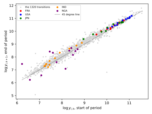
That naive reading would be a mistake, however, and it is worth being convinced of it right away. Income per capita is not a stationary variable: it grows, and nothing guarantees a priori that it reverts to anything. So take the extreme case of a world in which no country converges: each income follows a random walk, with the observed average growth and shocks of the observed dispersion, starting from the 1963 incomes. Then run the two regressions again.
dy = LY[1:, :] - LY[:-1, :]
drift, shock = dy.mean(), (dy - dy.mean(axis=0)).std()
chance = np.random.default_rng(5)
walk = []
for _ in range(1000):
    Y = LY[0] + np.vstack([np.zeros(N), np.cumsum(drift + chance.normal(0, shock, (K, N)), axis=0)])
    bf, af = Y[:-1, :], Y[1:, :]
    walk.append([slope(bf, af), slope(bf - bf.mean(axis=0), af - af.mean(axis=0))])
walk = np.array(walk)
print(walk.mean(axis=0).round(3), np.percentile(walk[:, 1], [5, 95]).round(3),
      (walk[:, 1] <= s_within).mean().round(2))
The pooled slope is 1.000 on average, and the within slope 0.906 — the two observed numbers, although these data contain no convergence at all. The within slope lies between 0.884 and 0.926 in 90% of cases, and the observed value sits in the middle of that distribution. In other words, the experiment cannot tell our data apart from a world without convergence. The remark below explains why subtracting a country's average mechanically lowers the slope, even when the true one is one, and an exercise gives the exact formula.
What the experiment shows is only that the two dimensions of the data give different answers, and that the within dimension cannot be read without care. To establish convergence, two things will be needed that this regression lacks: the determinants of each country's steady state, which the Solow model provides, and a correction of the bias, which will occupy most of the note.
A warning, to avoid a common misreading. The within transformation is harmless in a static panel: subtracting an average does not correlate the regressors with the error if those regressors are given in advance. It ceases to be harmless as soon as the lagged variable sits on the right hand side, because the average being subtracted also contains the disturbances of every period — including those that determined lagged income. The transformed regressor and the transformed error then become correlated. This is the Nickell bias, and it will occupy the section on the bias of the within estimator.
The within estimator
Let us move from the illustration to the model. The within transformation of the previous section subtracted from each country its time average; it will have to be generalised, because our equation is not that of an ordinary panel. Write \(r_{i,k}(\theta,\alpha)\) for the residual before the country unknown is removed, that is, whatever remains once the part predicted by the model has been subtracted. The equation then reads \(r_{i,k} = g_{i,k}\log A_i(0) + v_{i,k+1}\): the country unknown is indeed the same at every date, but it is multiplied by a coefficient \(g_{i,k}\) which changes from one period to the next. Subtracting the simple average would therefore not eliminate it. What is to be done? Read the equation \(r_{i,k} = g_{i,k}\log A_i(0) + v_{i,k+1}\) for what it is: a regression, country by country, of the residual \(r_{i,k}\) on the coefficient \(g_{i,k}\), and with no intercept. The unknown \(\log A_i(0)\) is its slope. For given \(\theta\) and \(\alpha\), minimising over \(\log A_i(0)\) therefore gives the ordinary least squares slope of \(r_{i,k}\) on \(g_{i,k}\):
\begin{equation*} \widehat{\log A_i(0)} = \frac{\sum_{k} g_{i,k}\,r_{i,k}}{\sum_{k} g_{i,k}^2} \end{equation*}and the concentrated criterion is the sum of squares of \(r_{i,k} - g_{i,k}\widehat{\log A_i(0)}\). It can also be read as a weighted average: dividing the equation by \(g_{i,k}\), each period offers the estimate \(r_{i,k}/g_{i,k}\), and the formula averages them with weight \(g_{i,k}^2\) — the periods in which the country converges fastest, those in which initial efficiency weighs most, count for more. When the rates are constant, \(g_{i,k}\) no longer depends on \(k\), the formula reduces to the time average of the residuals, and we recover the usual within transformation. It is therefore a generalisation, not another estimator.
The estimation itself is by non-linear least squares (NLS), as in the cross-section note: the sum of squares of these concentrated residuals is minimised over \(\theta\) and \(\alpha\), by a Gauss-Newton type algorithm — which at each iteration replaces the model by its linear approximation and applies OLS — started from several points. Since the equation is linear in \(\log A_i(0)\), concentrating out the 110 country unknowns in this way gives exactly the same estimates as NLS over all 112 parameters at once, for a problem in two dimensions only. The standard errors come from the usual NLS formula, \(\hat\sigma^2(J'J)^{-1}\), where \(J\) is the matrix of derivatives of the concentrated residuals with respect to the two parameters — the Jacobian, which plays here the role of the matrix of regressors, and the test of the constraint compares the sums of squared residuals with and without it.
This regression is not a matter of writing. Were one to subtract the simple average of the residuals while the coefficient of \(\log A_i(0)\) varies, the country unknown would not be eliminated, and the estimate would be wrong: \(\hat\theta\) would fall to 0.07. And it must be redone inside the function that computes the residuals: its regressor \(g_{i,k}\) depends on \(\theta\), so it changes at every iteration of the optimiser. Demeaning the data beforehand, as a linear-panel reflex would, gives a different estimator, and an incorrect one.
def raws(p, LY, S, C, K, tau, constrained=False):
    """Residuals r_{i,k} before the country unknown is removed, and coefficients g_{i,k}."""
    alpha = p[0] if constrained else p[1]
    theta = 1 - alpha if constrained else p[0]
    rho = np.exp(-theta*C*tau)
    tk = (np.arange(K)*tau)[:, None]
    pred = (rho*LY[:-1, :] + (1 - rho)*alpha/(1 - alpha)*(np.log(S) - np.log(C))
            + X*(tau + tk*(1 - rho)))
    return LY[1:, :] - pred, 1 - rho

def within(LY, S, C, K, tau, constrained=False):
    """NLS, log A_i(0) concentrated out by the regression of r on g."""
    def criterion(p):
        r, g = raws(p, LY, S, C, K, tau, constrained)
        return (r - g*(g*r).sum(axis=0)/(g*g).sum(axis=0)).ravel()
    if constrained:
        starts, bounds = [[0.4], [0.6], [0.8]], ([0.01], [0.99])
    else:
        starts, bounds = [[0.4, 0.4], [0.1, 0.7], [0.8, 0.2], [0.03, 0.5]], \
                         ([1e-4, 0.01], [5, 0.99])
    tries = [least_squares(criterion, p0, bounds=bounds) for p0 in starts]
    return min(tries, key=lambda e: e.cost)

def results(tau):
    """Free estimate, constrained estimate, standard errors and test."""
    A, B, Cx, Kx = panel(tau)
    f, fc = within(A, B, Cx, Kx, tau), within(A, B, Cx, Kx, tau, constrained=True)
    df = Kx*N - N - 2
    V = np.linalg.inv(f.jac.T @ f.jac)*(f.fun @ f.fun)/df
    sigma = np.sqrt(f.fun @ f.fun/((Kx - 1)*N))
    F = (2*fc.cost - 2*f.cost)/(2*f.cost/df)
    return f, np.sqrt(np.diag(V)), sigma, F, Kx, Cx

f, se, sigma, F, Kx, Cx = results(5)
print(Kx, f.x.round(4), se.round(4), np.median(f.x[0]*Cx.mean(axis=0)).round(4),
      sigma.round(4), round(F, 2), round(f.x[0] - (1 - f.x[1]), 3))
With five-year periods, the estimate is \(\hat\theta = 0.478\) (standard error 0.048) and \(\hat\alpha = 0.370\) (0.037), that is, a median convergence speed of 3.9% per year. This is more than four times the cross-section estimate, 0.86%, and the order of magnitude Islam (1995) reports. The constraint of the full Solow model, \(\theta = 1-\alpha\), is rejected: the F statistic is 12.6.
y = LY[1:, :].ravel()
D = np.tile(np.eye(N), (K, 1))
T = np.repeat(np.eye(K)[:, 1:], N, axis=0)
Z = np.column_stack([LY[:-1, :].ravel(), np.log(S).ravel(), np.log(C).ravel(), D, T])
b = np.linalg.lstsq(Z, y, rcond=None)[0]
print(b[0], -np.log(b[0])/5, b[1], b[1]/(1 - b[0] + b[1]))

def fit(e, k):
    """SSR, R² on within growth, AIC and BIC of a specification with k parameters."""
    dy_within = (LY[1:, :] - LY[:-1, :]) - (LY[1:, :] - LY[:-1, :]).mean(axis=0)
    ssr, n = e @ e, e.size
    ll = -n/2*np.log(ssr/n)
    return [round(ssr, 2), k, round(1 - ssr/(dy_within**2).sum(), 3),
            round(-2*ll + 2*k, 1), round(-2*ll + k*np.log(n), 1)]

r_s, g_s = raws(results(5)[0].x, LY, S, C, K, 5)
e_s = (r_s - g_s*(g_s*r_s).sum(axis=0)/(g_s*g_s).sum(axis=0)).ravel()
Z0 = Z[:, :3 + N]
b0 = np.linalg.lstsq(Z0, y, rcond=None)[0]
print(fit(e_s, 2 + N))
print(fit(y - Z @ b, Z.shape[1]))
print(fit(y - Z0 @ b0, Z0.shape[1]), round(b0[0], 3))
As a benchmark, the usual linear regression, the one that treats \(\rho\) as a common coefficient and adds country and period dummies, gives \(\hat\rho = 0.842\), that is 3.4% per year, and an implied capital share of 0.44.
Comparing the fit of the two approaches is instructive, provided one separates what distinguishes them. The table reports the sum of squared residuals (SSR), the share of the within variation of the growth rate that is explained, and two information criteria that penalise the number of parameters, Akaike's (AIC) and Schwarz's (BIC): the lower they are, the better the specification.
| specification | parameters | SSR | \(R^2\) | AIC | BIC |
|---|---|---|---|---|---|
| structural | 112 | 50.99 | 0.102 | −4071.0 | −3490.2 |
| linear, country and period dummies | 124 | 45.51 | 0.199 | −4197.2 | −3554.2 |
| linear, country dummies only | 113 | 50.62 | 0.109 | −4078.5 | −3492.6 |
The usual regression fits clearly better: its SSR is 11% lower, and both criteria prefer it. But the last row shows where the gap comes from. Without period dummies, the linear regression, which leaves the coefficients of \(\log s\) and \(\log c\) free, fits no better than the structural model, and its \(\hat\rho\) rises to 0.884. Imposing the Solow structure instead of free coefficients therefore costs almost nothing, and buys a test. What does cost is replacing shocks common to each period by the deterministic trend of the model. The section on the limits of the statistical model will come back to this.
f5b = results(5)[0]
r5b, g5b = raws(f5b.x, LY, S, C, K, 5)
e5b = r5b - g5b*(g5b*r5b).sum(axis=0)/(g5b*g5b).sum(axis=0)
for aim in (LY[1:, :], LY[1:, :] - LY[:-1, :]):
    within_aim = aim - aim.mean(axis=0)
    print(round(1 - (e5b*e5b).sum()/(within_aim*within_aim).sum(), 3))
Here is the one place where the level form and the growth form are not equivalent, and it is worth flagging. The residuals are the same, but the share of variation explained depends on what one claims to explain: measured against the within variation of the level it is 0.84, whereas the table above, measured against the growth rate, gave 0.10. The first number says nothing about the model — income is so persistent that predicting the next period's level is almost free — and would flatter any specification. The second is the honest one, and it is modest. This is why an \(R^2\) only makes sense, in a dynamic panel, relative to the quantity the model actually claims to explain.
The bias of the within estimator
It remains to know what \(\hat\theta = 0.478\) is worth. Subtracting from each country its weighted average, in an equation where lagged income sits on the right hand side, correlates the transformed regressor with the transformed error: this is the bias Nickell (1981) computed for the linear model, of order \(-(1+\rho)/(K-1)\) on \(\rho\), and the note on the bias of the least squares estimator of an AR(1) process explains the mechanism. A \(\hat\rho\) that is too small is a speed that is too large. But Nickell's order of magnitude assumes a linear model, and it will prove far too optimistic.
We can measure this bias by simulation. The model provides its own data generating process: pick \(\theta\), \(\alpha\), the standard deviation \(\sigma\) of the disturbances, the moving-average parameter \(\psi\) introduced below, and the efficiencies \(\log A_i(0)\), start from the incomes observed in 1963, and apply the equation period after period. The efficiencies are still missing: we recover them from the estimation by the same regression of \(r_{i,k}\) on \(g_{i,k}\), the one that concentrated them out of the criterion.
f5 = within(LY, S, C, K, 5)
theta5, alpha5 = f5.x
r5, g5 = raws(f5.x, LY, S, C, K, 5)
lA0 = (g5*r5).sum(axis=0)/(g5*g5).sum(axis=0)
cbar = C.mean(axis=0)
print(lA0.std().round(3), np.median(cbar).round(4))
They are widely dispersed across countries — a standard deviation of 1.11 in logarithms, that is a factor of three between a typically efficient country and another — and in the simulations we shall treat them as given characteristics, on the same footing as the observed rates.
def simulate(theta, alpha, sigma, psi, lA0, LY, S, C, K, tau, rng):
    """A panel simulated by the model, MA(1) errors, given efficiencies and initial incomes."""
    rho = np.exp(-theta*C*tau)
    g = 1 - rho
    Z = g*(alpha/(1 - alpha)*(np.log(S) - np.log(C)) + lA0)
    eps = rng.normal(0, sigma, (K + 1, len(lA0)))
    v = eps[1:] + psi*eps[:-1]
    Y = np.empty_like(LY)
    Y[0] = LY[0]
    for k in range(K):
        Y[k+1] = rho[k]*Y[k] + Z[k] + X*(tau + k*tau*g[k]) + v[k]
    return Y

def expectation(theta, alpha, sigma, psi, lA0, LY, S, C, K, tau, B, rng):
    """Average of the within estimator over B simulated panels."""
    return np.array([within(simulate(theta, alpha, sigma, psi, lA0, LY, S, C, K, tau, rng),
                            S, C, K, tau).x for _ in range(B)])
The standard deviation of the disturbances estimated on the data is 0.20, and it is at that level that the experiment makes sense: an estimator may well be excellent in a nearly deterministic world and mute in ours. Let us also be clear about what we are after here. It is not the consistency of the estimator, which is about what happens at a given standard deviation as the sample grows, and which is the subject of the last of the exercises; it is its bias at the size of our sample, 110 countries and twelve periods.
The table below gives the experiment at the noise level of the data. Two values in it are borrowed from the next section, for want of anything better: the capital share, \(\alpha = 0.508\), and the moving-average parameter, \(\psi = 0.294\), both estimated further on. Simulating requires a complete set of parameters, and these are the only ones we shall have.
GRID = (0.10, 0.176, 0.30, 0.60)
dice_bias = np.random.default_rng(2014)
curve = {th: expectation(th, 0.508, 0.2045, 0.294, lA0, LY, S, C, K, 5, 200, dice_bias)
         for th in GRID}
for th in GRID:
    print(th, curve[th][:, 0].mean().round(3), curve[th][:, 0].std().round(3))
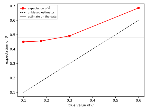
| true \(\theta\) | 0.10 | 0.176 | 0.30 | 0.60 |
| \(\mathbb{E}[\hat\theta]\) | 0.451 | 0.456 | 0.492 | 0.686 |
The curve is flat: between 0.10 and 0.176 — the range in which, as we shall see, the maximum likelihood estimate falls — the expectation of \(\hat\theta\) barely moves, and one has to triple the true value to see it rise from 0.451 to 0.492. Over that whole range the within estimator distinguishes nothing. This is no longer a bias one would correct by subtracting a constant, it is a statistic that barely responds to the parameter. The standard error of \(\hat\theta\), 0.048, carries no information in these conditions.
An estimator by maximum likelihood
Since the within estimator barely responds to the parameter, another one is needed. The classic way of getting rid of a fixed effect without subtracting an average is to difference: compare each period with the previous one rather than with the average of all. But here the simple difference \(r_{i,k} - r_{i,k-1}\) does not remove the country unknown, since its coefficient changes from one period to the next. Let us therefore proceed in two steps, slowly, for this is the technical heart of the note.
First step, normalise. Divide each residual by its own coefficient:
\begin{equation*} u_{i,k} \equiv \frac{r_{i,k}}{g_{i,k}} = \log A_i(0) + \frac{v_{i,k+1}}{g_{i,k}} \end{equation*}The country unknown now appears with the same coefficient, one, in every period; in exchange the error has been distorted, and its variance is now \(\sigma^2 h_{i,k}\) with \(h_{i,k} = 1/g_{i,k}^2\).
Second step, difference. The successive gaps \(z_{i,k} = u_{i,k} - u_{i,k-1}\) no longer contain \(\log A_i(0)\) at all, for \(k = 2,\ldots,K\). This is, up to a factor \(1/g_{i,k}\), the quasi-difference \(r_{i,k} - (g_{i,k}/g_{i,k-1})\,r_{i,k-1}\) that Holtz-Eakin, Newey and Rosen (1988) proposed for fixed effects with varying coefficients. That leaves \(K-1\) quantities rid of the unknown, and a first observation, \(z_{i,1} = r_{i,1}\), which still contains it. Rather than discard it, we follow Hsiao, Pesaran and Tahmiscioglu (2002): we give it a free mean — projected on the initial saving rate and on \(\log c_{i,1}\) — and a free variance \(\omega\sigma^2\), which absorbs what we do not know about the initial condition.
Third step, say what is assumed about the errors. Independence of the \(v_{i,k}\) would be convenient, but the way the data are built makes it implausible. Saving and depreciation rates are period averages, and gross domestic product is itself a flow measured over the year: our observations are therefore temporal aggregates, and averaging a flow creates a positive correlation between neighbouring periods, even when the underlying process has none. This is an old result, due to Working (1960), which gives +0.25 at the first lag for an aggregated random walk. Rather than impose independence, let us give the model the corresponding freedom, that of a first-order moving average:
\begin{equation*} v_{i,k} = \varepsilon_{i,k} + \psi\,\varepsilon_{i,k-1},\qquad \varepsilon_{i,k} \sim \mathcal{N}(0,\sigma^2)\ \text{independent} \end{equation*}so that \(\mathbb{V}(v) = \sigma^2(1+\psi^2)\) and \(\mathrm{Cov}(v_{i,k},v_{i,k-1}) = \sigma^2\psi\). Independence remains the special case \(\psi = 0\), and the data will say what it is.
Let us now write the distribution of the vector \(z_i = (z_{i,1},\ldots,z_{i,K})\). The two operations, normalising then differencing, are linear: writing \(T_i\) for the matrix that leaves the first row intact and forms the gaps \(r_{i,k}/g_{i,k} - r_{i,k-1}/g_{i,k-1}\) for \(k\geq2\), we have \(z_i = T_i\,r_i\), and therefore
\begin{equation*} \mathbb{V}(z_i) = \sigma^2\Sigma_i,\qquad \Sigma_i = T_i\,V\,T_i'\ \text{ where }\ V = \begin{pmatrix} 1+\psi^2 & \psi & & \\ \psi & 1+\psi^2 & \psi & \\ & \psi & 1+\psi^2 & \ddots \\ & & \ddots & \ddots \end{pmatrix} \end{equation*}is the covariance of the \(v\), up to \(\sigma^2\). Only one entry escapes this formula: that of the first observation, whose variance is the free parameter \(\omega\sigma^2\) rather than what the model would predict. The easiest way to read this matrix is to look at the case \(\psi = 0\), where it is tridiagonal:
\begin{equation*} \Sigma_i = \begin{pmatrix} \omega & -1/g_{i,1} & & \\ -1/g_{i,1} & h_{i,2}+h_{i,1} & -h_{i,2} & \\ & -h_{i,2} & h_{i,3}+h_{i,2} & \ddots \\ & & \ddots & \ddots \end{pmatrix} \end{equation*}Each gap shares an error with its neighbour, hence the off-diagonal terms, and the matrix is specific to each country since the \(h\) are. With \(\psi \neq 0\) the errors overlap by one further period and \(\Sigma_i\) ceases to be tridiagonal, without anything changing in the construction. The log-likelihood follows. Replacing \(\sigma^2\) by the estimator that maximises it, \(\hat\sigma^2 = \frac{1}{NK}\sum_i z_i'\Sigma_i^{-1}z_i\), gives the concentrated criterion
\begin{equation*} \ell(\theta,\alpha,\omega,\psi) = -\frac{NK}{2}\log\hat\sigma^2(\theta,\alpha,\omega,\psi) - \frac{1}{2}\sum_{i}\log|\Sigma_i| + \sum_{i}\sum_{k\geq2}\log g_{i,k} \end{equation*}which we maximise numerically.
The last term is the easiest to forget, and forgetting it ruins everything. We have replaced the data \(r\) by quantities \(z\) derived from them, and the density of a transformed variable involves the Jacobian of the transformation. Here the transformation divides rows \(2\) to \(K\) by \(g_{i,2},\ldots,g_{i,K}\), so its determinant is \(\prod_{k\geq2} 1/g_{i,k}\) and the log-likelihood of the data gains \(+\sum_{k\geq2}\log g_{i,k}\). That term depends on \(\theta\), since \(g_{i,k} = 1-e^{-\theta c_{i,k}\tau}\). Without it the optimiser discovers that it can improve the criterion by moving \(\theta\) so as to inflate the \(g\), explaining nothing more, and the estimate then runs to the upper boundary. When the rates are constant, this term and the division by \(g\) cancel each other exactly, and we recover the usual first-difference likelihood.
def unpack(q):
    """(theta, alpha, omega, psi) from unconstrained parameters."""
    return (np.exp(q[0]), 0.01 + 0.98/(1 + np.exp(-q[1])), np.exp(q[2]), 0.95*np.tanh(q[3]))

def covariance_ma(psi, K):
    """Covariance of the errors, up to sigma^2: gamma_h = sum_j psi_j psi_{j+h}."""
    p = np.concatenate([[1.0], np.atleast_1d(psi)])
    V = np.zeros((K, K))
    for h in range(len(p)):
        gh = float(np.dot(p[:len(p)-h], p[h:]))
        V += np.eye(K, k=h)*gh + (np.eye(K, k=-h)*gh if h else 0)
    return V

def pieces(theta, alpha, omega, psi, LY, S, C, K, tau, projected=True):
    """Transformed vector z and its covariance Sigma, stacked over countries, up to sigma^2."""
    r, g = raws([theta, alpha], LY, S, C, K, tau)
    if np.any(g <= 1e-8):
        return None, None, None
    n = r.shape[1]
    V = covariance_ma(psi, K)
    T = np.zeros((n, K, K))
    T[:, 0, 0] = 1
    for k in range(1, K):
        T[:, k, k], T[:, k, k-1] = 1/g[k], -1/g[k-1]
    Sigma = T @ V @ np.transpose(T, (0, 2, 1))
    Sigma[:, 0, 0] = omega
    z = np.empty((n, K))
    z[:, 0] = r[0]
    z[:, 1:] = (r[1:]/g[1:] - r[:-1]/g[:-1]).T
    W = (np.column_stack([np.ones(n), np.log(S[0]), np.log(C[0])]) if projected
         else np.ones((n, 1)))
    z[:, 0] = z[:, 0] - W @ np.linalg.lstsq(W, z[:, 0], rcond=None)[0]
    return z, Sigma, g

def criterion(theta, alpha, omega, psi, LY, S, C, K, tau, projected=True):
    """Concentrated criterion, Jacobian included (sign flipped, to be minimised)."""
    if theta > 5 or omega > 1e6 or omega < 1e-6:
        return 1e10
    z, Sigma, g = pieces(theta, alpha, omega, psi, LY, S, C, K, tau, projected)
    if z is None:
        return 1e10
    try:
        L = np.linalg.cholesky(Sigma)
    except np.linalg.LinAlgError:
        return 1e10
    y = np.linalg.solve(L, z[:, :, None])[:, :, 0]
    quad = np.sum(y*y)
    if quad <= 0:
        return 1e10
    ldet = 2*np.sum(np.log(np.diagonal(L, axis1=1, axis2=2)))
    n = z.shape[0]
    return K*n/2*np.log(quad/(K*n)) + 0.5*ldet + np.sum(np.log(g[1:]))

def loglik(q, LY, S, C, K, tau, projected=True):
    """The same criterion, from unconstrained parameters."""
    return criterion(*unpack(q), LY, S, C, K, tau, projected)

def start(theta, alpha, omega=1.2, psi=0.25):
    a = (alpha - 0.01)/0.98
    return [np.log(theta), np.log(a/(1 - a)), np.log(omega), np.arctanh(psi/0.95)]

def mle(LY, S, C, K, tau, projected=True,
        starts=((0.2, 0.55, 1.2, 0.25), (0.4, 0.4, 1.2, 0.0), (0.1, 0.7, 1.2, 0.4))):
    """Maximum likelihood, several starting points."""
    tries = [minimize(loglik, start(*p), args=(LY, S, C, K, tau, projected),
                      method='Nelder-Mead', options=dict(maxiter=4000, xatol=1e-7, fatol=1e-9))
             for p in starts]
    return unpack(min(tries, key=lambda e: e.fun).x)

def sd_of(theta, alpha, omega, psi, LY, S, C, K, tau):
    """Standard deviation of the innovations, concentrated out of the likelihood."""
    z, Sigma, _ = pieces(theta, alpha, omega, psi, LY, S, C, K, tau)
    L = np.linalg.cholesky(Sigma)
    y = np.linalg.solve(L, z[:, :, None])[:, :, 0]
    return np.sqrt(np.sum(y*y)/(K*z.shape[0]))

for projected in (False, True):
    print(projected, np.round(mle(LY, S, C, K, 5, projected), 4))
free_ll = loglik(start(*mle(LY, S, C, K, 5)), LY, S, C, K, 5)
null_ll = minimize(lambda q: loglik([q[0], q[1], q[2], np.arctanh(0.0)], LY, S, C, K, 5),
                   start(0.2, 0.55)[:3], method='Nelder-Mead').fun
print('psi = 0 imposed:', round(null_ll - free_ll, 1), round(2*(null_ll - free_ll), 1))
The choice of the mean of that first observation is decisive, and this is the whole point of the exercise. Giving it a mean common to all countries yields \(\hat\theta = 0.027\) and \(\hat\alpha = 0.801\), that is, even less than the cross-section estimate: by assuming the initial condition independent of the regressors, one has reintroduced exactly the endogeneity the panel was meant to remove. Projecting it on the initial saving rate and on \(\log c_{i,1}\) yields \(\hat\theta = 0.176\), \(\hat\alpha = 0.508\) and \(\hat\omega = 1.27\). All the information about levels is in the initial condition, and that is where the endogeneity sits.
As for the moving-average parameter, it confirms what aggregation led us to expect: \(\hat\psi = 0.29\), an order of magnitude close to Working's +0.25, and imposing it to be zero worsens the criterion by 51 points, that is a likelihood ratio of 102 for a single degree of freedom — twice the gap in the criterion, the quantity whose distribution the \(\chi^2\) tabulates when the constraint holds. The freedom we gave the errors was therefore no stylistic precaution, and the section on the limits will establish that aggregation is indeed its cause.
It has to be said plainly: the proof of Hsiao, Pesaran and Tahmiscioglu assumes a \(\rho\) common to all countries, whereas here \(\rho_{i,k}\) varies in both dimensions. Nothing guarantees that their consistency result applies as it stands. We shall not invoke it: the quality of this estimator will be judged on the Monte Carlo, like that of the previous one. Note in passing that a low-noise recovery test, decisive for the within estimator, says nothing about this one: as \(\sigma\) tends to zero the contrasts vanish identically, whatever the value of \(\theta\). This estimator draws its information from the covariance structure of the contrasts, not from their expectation.
Correcting the bias by simulation
So let us put the new estimator through the same test.
theta_ml, alpha_ml, omega_ml, psi_ml = mle(LY, S, C, K, 5)
sigma_ml = sd_of(theta_ml, alpha_ml, omega_ml, psi_ml, LY, S, C, K, 5)
def efficiencies(theta, alpha, LY, S, C, K, tau):
    """Initial efficiencies: no-intercept regression of r on g, at given θ and α."""
    r, g = raws([theta, alpha], LY, S, C, K, tau)
    return (g*r).sum(axis=0)/(g*g).sum(axis=0)

lA0_ml = efficiencies(theta_ml, alpha_ml, LY, S, C, K, 5)

def expectation_ml(theta, alpha, sigma, psi, LY, S, C, K, tau, B, rng):
    """Average of the MLE over B simulated panels, efficiencies implied by θ and α."""
    lA0 = efficiencies(theta, alpha, LY, S, C, K, tau)
    return np.array([mle(simulate(theta, alpha, sigma, psi, lA0, LY, S, C, K, tau, rng),
                         S, C, K, tau, starts=((theta, alpha, omega_ml, psi),))[:2]
                     for _ in range(B)])

dice_bind = np.random.default_rng(2015)
curve_ml = {th: expectation_ml(th, 0.508, sigma_ml, psi_ml, LY, S, C, K, 5, 40, dice_bind)
            for th in GRID}
for th in GRID:
    print(th, curve_ml[th][:, 0].mean().round(3))
| true \(\theta\) | 0.10 | 0.176 | 0.30 | 0.60 |
| \(\mathbb{E}[\hat\theta_{\text{ML}}]\) | 0.093 | 0.129 | 0.182 | 0.484 |
It is biased too, and downwards, by a factor that is anything but constant: 7% at \(\theta = 0.10\), 27% at the level of the observed estimate, 39% at \(\theta = 0.30\), then 19% at \(\theta = 0.60\). But, unlike the previous one, it is monotone, and clearly increasing: to each value of its expectation there corresponds a single value of the parameter. That is enough to correct it, by a method called indirect inference. It resembles nothing one usually does in econometrics, and deserves to be taken step by step.
The idea. Imagine a scale that does not weigh correctly, without our knowing by how much it errs. It can be calibrated: put on it weights whose mass is known, note what it displays, and draw the curve of the display as a function of the true mass. To weigh an unknown object afterwards, read the display, look on the curve for the mass that produces it, and retain that mass. The scale has not been repaired; we have only learnt to read it. Our estimator is the scale, and the known weights are simulated panels: for a chosen value of \(\theta\), we simulate the model many times, apply the estimator to each panel, and average. This gives, point by point, the function
\begin{equation*} b(\theta) = \mathbb{E}_{\theta}\bigl[\hat\theta\bigr] \end{equation*}which Gouriéroux, Monfort and Renault (1993) call the binding function — it is exactly the row of the table above. An unbiased estimator would have \(b(\theta) = \theta\). Ours does not, but it does not matter: we retain the value \(\theta^{\star}\) that would have produced, on average, the estimate obtained on the real data,
\begin{equation*} b(\theta^{\star}) = \hat\theta_{\text{obs}} \end{equation*}Graphically, start from \(\hat\theta_{\text{obs}} = 0.176\) on the vertical axis, move horizontally to the curve, and read off the abscissa.
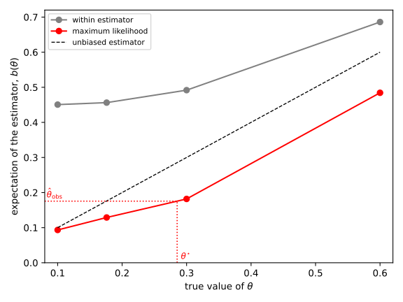
The graphical reading, at fixed \(\alpha\), already gives \(\theta^{\star}\approx 0.29\).
What is needed, and what is not. The method requires three things. First, one must be able to simulate the model for any value of the parameters; this is the case, the equation of the model provides its own generator. Second, one must apply to the simulated data exactly the same estimator as to the real data, with the same 1963 incomes, the same rates and the same partition of time: this is what guarantees that the bias, whatever its source, strikes both in the same way, and cancels out when they are compared. Third, the binding function must be strictly monotone, and steep enough: where it is flat, a small change in the observed estimate corresponds to a large change in the parameter, and the inversion no longer makes sense. On the other hand — and this is what surprises at first — it is not necessary for the estimator being inverted, called the auxiliary estimator, to be unbiased, or even consistent. It need not be good, only informative. This is why the within estimator, whose curve is flat, cannot serve, whereas maximum likelihood, biased as it is too, can. Gouriéroux, Phillips and Yu (2010) applied the method to dynamic panels by inverting the within estimator; in their linear model it is steep, in ours it is not.
With two parameters. The correction cannot be made at fixed \(\alpha\), because the estimator of \(\alpha\) is biased too, and its bias depends on \(\theta\). The binding function therefore associates a pair of expectations \((\mathbb{E}[\hat\theta],\mathbb{E}[\hat\alpha])\) with each pair \((\theta,\alpha)\), and a system of two equations in two unknowns must be solved. It can no longer be read on a graph, but it is solved by iteration. Starting from \(p_0 = (\hat\theta_{\text{obs}},\hat\alpha_{\text{obs}})\), we compute
\begin{equation*} p_{j+1} = p_j + \lambda\bigl(\hat p_{\text{obs}} - \hat b(p_j)\bigr) \end{equation*}where \(\hat b(p_j)\) is the average of the estimates over \(B\) panels simulated with the parameters \(p_j\). One clarification is in order about what \(p_j\) contains: the iteration runs on \(\theta\) and \(\alpha\) only, but the 110 efficiencies are nonetheless refreshed at every step. They are not extra unknowns: at given \(\theta\) and \(\alpha\) they can be read off the data, by the no-intercept regression of \(r_{i,k}\) on \(g_{i,k}\), the very one that concentrates the likelihood. Freezing them at the uncorrected point would amount to simulating a world whose efficiencies contradict its own speed of convergence, and we shall see below that this is no mere matter of wording. What does stay fixed is the standard deviation of the disturbances, the variance of the first observation and the moving-average parameter; for \(\sigma\), which also has a closed form once \(\omega\) and \(\psi\) are given, refreshing it does not move \(\theta^{\star}\) beyond the third decimal. One further clarification: the bias curves drawn above, computed before maximum likelihood was built, use the efficiencies of the within estimator. The first iteration is the bias correction anyone would make spontaneously: measure the bias at the estimated point and subtract it. If the bias were the same for every value of the parameter, it would be enough. It is not — from 7 to 39% depending on the target — and the following iterations correct the correction, until the simulated parameters reproduce the observed estimate. The coefficient \(\lambda = 0.9\) damps the oscillations due to simulation noise.
def correction(aim, sigma, psi, LY, S, C, K, tau, rng,
               iterations=20, B=40, step=0.9, keep=8):
    """θ and α such that the simulated estimator reproduces the observed estimate."""
    p, path = np.array(aim, dtype=float), []
    for _ in range(iterations):
        out = expectation_ml(p[0], p[1], sigma, psi, LY, S, C, K, tau, B, rng).mean(axis=0)
        p = p + step*(np.array(aim) - out)
        p = np.array([min(max(p[0], 1e-3), 3), min(max(p[1], 0.05), 0.95)])
        path.append(p.copy())
    return np.mean(path[-keep:], axis=0)          # tail average, against simulation noise

star = correction([theta_ml, alpha_ml], sigma_ml, psi_ml, LY, S, C, K, 5,
                  np.random.default_rng(2016))
lA0_star = efficiencies(*star, LY, S, C, K, 5)
print(star.round(3), np.median(star[0]*cbar).round(4), (star[0] - (1 - star[1])).round(3))
The correction gives \(\theta^{\star} = 0.36\) and \(\alpha^{\star} = 0.32\), that is, a median convergence speed of 2.9% per year: the corrected parameter is twice the raw estimate. Note that the correction also moves the capital share, from 0.51 to 0.32: this is why reading the bias curve at a fixed \(\alpha\) would not have been enough, and why the fixed point is taken over both parameters at once.
How precise? Since \(p^{\star} = b^{-1}(\hat p_{\text{obs}})\), the uncertainty on \(\hat p_{\text{obs}}\) is passed on to \(p^{\star}\) through the inverse of the binding function. To first order, if \(J\) denotes the matrix of derivatives of \(b\) and \(V\) the variance matrix of the auxiliary estimator, both evaluated at \(p^{\star}\),
\begin{equation*} \mathbb{V}\bigl(p^{\star}\bigr) \simeq \Bigl(1+\frac{1}{B}\Bigr)J^{-1}\,V\,{J^{-1}}' \end{equation*}This is the delta method, that is, the propagation of an uncertainty through a function replaced by its tangent, here that of the inverse of \(b\). The factor \(1+1/B\) accounts for \(b\) being known only through \(B\) simulations, and it is the \(B\) of the correction, forty, that enters here. The formula also says, in one line, why the slope matters: dividing by a derivative close to zero, that of the within estimator, would make the variance infinite. Both ingredients are again obtained by simulation, \(V\) by repeating the estimation at \(p^{\star}\), \(J\) by finite differences, reusing the same draws on either side of the point so that simulation noise is not mistaken for slope.
seed, h, Bp = 1, 0.03, 60
base = expectation_ml(*star, sigma_ml, psi_ml, LY, S, C, K, 5, Bp,
                      np.random.default_rng(seed))
J = np.empty((2, 2))
for j in range(2):
    step_j = h*np.eye(2)[j]
    up, down = (expectation_ml(*(star + sign*step_j), sigma_ml, psi_ml, LY, S, C, K,
                               5, Bp, np.random.default_rng(seed)).mean(axis=0)
                for sign in (1, -1))
    J[:, j] = (up - down)/(2*h)
Ji = np.linalg.inv(J)
se_star = np.sqrt(np.diag((1 + 1/40)*Ji @ np.cov(base.T) @ Ji.T))
print(J.round(2), se_star.round(3),
      (np.median(cbar)*(star[0] + np.array([-1.645, 1.645])*se_star[0])).round(4))
And this is where the correction shows its price. The slope of \(\mathbb{E}[\hat\theta]\) with respect to \(\theta\) is only 0.53: doubling the true speed moves the auxiliary estimator by only half as much, so that the inverse reading doubles every uncertainty. The standard error of \(\theta^{\star}\) is 0.167, that of \(\alpha^{\star}\) 0.134, and the 90% confidence interval of the median speed runs from 0.7 to 5.2% per year. That is wide, and it should be said as such: the data place the speed above what the raw estimate displays, but they do not place it precisely.
A word on what the easy way would cost. Freezing the efficiencies at the uncorrected point, instead of recomputing them, would show a slope of 1.17 and a standard error of 0.038 — a precision four times better, and entirely illusory. It comes from the freeze preventing the efficiencies from responding to \(\theta\): the binding function then looks three times steeper than it is, and its inversion far better determined.
The Solow constraint, \(\theta = 1-\alpha\), can then be tested without invoking any asymptotic distribution, by simulating under the constraint.
under_h0 = expectation_ml(1 - star[1], star[1], sigma_ml, psi_ml, LY, S, C, K, 5,
                          150, np.random.default_rng(2017))
gap0 = under_h0[:, 0] - (1 - under_h0[:, 1])
gap = theta_ml - (1 - alpha_ml)
print(gap0.mean().round(3), np.percentile(gap0, [5, 95]).round(3),
      round(gap, 3), (gap0 <= gap).mean())
Under the null, the gap \(\hat\theta - (1-\hat\alpha)\) is not centred — it averages −0.109, since the two estimates that compose it are themselves biased — and lies in [−0.224; +0.016] in 90% of samples. That is precisely why the test is simulated rather than read off a table. The observed gap is −0.316, and no simulated sample reaches it: the full Solow model is rejected. This time the verdict does not rest on a \(\chi^2\) approximation which the section on the bias has shown to be worthless here.
A more elementary question comes first, however, and the section What a panel adds to a cross-section made it pressing: is there convergence at all? Income per capita is not stationary, and we have seen that a random walk, which converges to nothing, reproduces exactly the within slope of the data. Let us therefore put maximum likelihood through the same test. Simulate worlds without convergence — each income follows a random walk, with a drift common to all countries or specific to each, and, in the second case, the correlated errors of our model — and estimate the model on each of them.
no_convergence = np.random.default_rng(11)
shock_rw = (dy - dy.mean(axis=0)).std()

def world_without_convergence(own, psi):
    """Random walks calibrated on the data: common drift or country-specific drift."""
    e = no_convergence.normal(0, shock_rw/np.sqrt(1 + psi*psi), (K + 1, N))
    step_rw = (dy.mean(axis=0) if own else dy.mean()) + e[1:] + psi*e[:-1]
    return LY[0] + np.vstack([np.zeros(N), np.cumsum(step_rw, axis=0)])

for own, psi in ((False, 0.0), (True, psi_ml)):
    R = []
    for _ in range(300):
        Y = world_without_convergence(own, psi)
        R.append([mle(Y, S, C, K, 5)[0], within(Y, S, C, K, 5).x[0]])
    R = np.array(R)
    print(own, R[:, 0].mean().round(3), np.percentile(R[:, 0], 99).round(3),
          (R[:, 0] >= theta_ml).mean(), R[:, 1].mean().round(3),
          np.median(R[:, 1].mean()*cbar).round(4))
The verdict is unambiguous. In a world without convergence, maximum likelihood gives on average \(\hat\theta = 0.025\) with a common drift, 0.058 with country-specific drifts, and exceeds 0.10 and 0.13 respectively in only 1% of cases. Out of 600 simulated panels, none reaches the value obtained on the data, 0.176. Unlike the within estimator, maximum likelihood therefore tells our data apart from a world without convergence; and the within estimator, applied to the same panels, finds on average 0.63 and 0.23 there, that is, median speeds of 5.2 and 1.9% per year where there is none — figures nobody would hesitate to publish, which shows well enough that a plausible value is not a proof. The convergence this note measures is not an artefact of the non-stationarity of income. This test nonetheless has a limited reach: it rules out the random walk, not every form of non-convergence, and in particular not country-specific deterministic trends, which we have not simulated.
reconciled = expectation(theta_ml, alpha_ml, sigma_ml, psi_ml, lA0_ml, LY, S, C, K, 5,
                         400, np.random.default_rng(2019))[:, 0]
print(reconciled.mean().round(3), np.percentile(reconciled, [5, 95]).round(3),
      theta5.round(3), (reconciled >= theta5).mean().round(3))
Here is the most demanding test one can put the whole construction through. Simulate the model with the parameters estimated by maximum likelihood, and apply the within estimator to the data so produced: over 400 replications it gives 0.387 on average, and falls between 0.314 and 0.471 in 90% of cases. The within estimate obtained on the real data is 0.478 — above, barely, but above: the model produces a value at least as large in 3.5% of samples.
This result must be read both ways. On the one hand, most of the gap between 0.18 and 0.48 is indeed explained: a single value of \(\theta\), seen through two estimators, produces two numbers that everything seemed to set against each other — and the section Back to the cross-section will make the same demonstration for the cross-section estimate. On the other hand, the reconciliation is not perfect. The model struggles to generate a within estimate as high as the one in the data; something in the behaviour of the biased estimator is therefore not quite reproduced by our specification.
Is it really labour efficiency that we measure?
The panel delivers an estimate of \(\log A_i(0)\) for each of the 110 countries: in principle a valuable by-product, since it is the level of labour efficiency in 1963, which the cross-section could only absorb into a disturbance. It remains to check that this number measures what its name promises.
The comparison calls for a precaution. Our \(A\) augments labour, in Harrod's sense: \(Y = K^{\alpha}(AL)^{1-\alpha}\). The Penn World Tables publish a total factor productivity in Hicks's sense, `ctfp`, defined by \(Y = A_H K^{\alpha}(hL)^{1-\alpha}\) where \(h\) is human capital per person. These are not the same object. Equating the two expressions,
\begin{equation*} A^{1-\alpha} = A_H\,h^{1-\alpha} \qquad\Longleftrightarrow\qquad \log A = \frac{\log A_H}{1-\alpha} + \log h \end{equation*}so that the empirical counterpart of our estimate is not \(\log\) `ctfp`, but \(\log\) `ctfp` divided by \(1-\alpha\), plus the logarithm of human capital. With \(\hat\alpha = 0.51\) — the uncorrected value, the one at which the \(\log\hat A_i(0)\) were estimated — the divisor is about 2: differences in total factor productivity are doubled when expressed as labour efficiency.
measures = (pwt[pwt['year'] == START].set_index('countrycode')
            .reindex(codes)[['ctfp', 'hc']])
good = ((measures['ctfp'] > 0) & measures['hc'].notna()).to_numpy()
target = np.log(measures['ctfp'].to_numpy(float)[good])/(1 - alpha_ml) \
    + np.log(measures['hc'].to_numpy(float)[good])
ours = lA0_ml[good]
ranks = lambda v: np.argsort(np.argsort(v))
hc = np.log(measures['hc'].to_numpy(float)[good])
print(np.corrcoef(ours, hc)[0, 1].round(3))      # link with human capital
print(good.sum(), np.corrcoef(ours, target)[0, 1].round(3),
      np.corrcoef(ranks(ours), ranks(target))[0, 1].round(3),
      np.polyfit(target, ours, 1)[0].round(3), target.std().round(3), ours.std().round(3))
u, iu = list(np.array(codes)[good]), list(np.array(codes)[good]).index('USA')
for country in ('JPN', 'IND'):
    i = u.index(country)
    print(country, np.exp(target[i] - target[iu]).round(2), np.exp(ours[i] - ours[iu]).round(2))

def norm1(x, y):
    """Line minimising the sum of absolute deviations, less sensitive to isolated points."""
    return minimize(lambda p: np.abs(y - p[0] - p[1]*x).sum(), np.polyfit(x, y, 1)[::-1],
                    method='Nelder-Mead', options=dict(xatol=1e-8, fatol=1e-10)).x

ols, l1 = np.polyfit(target, ours, 1)[0], norm1(target, ours)[1]
dropped = np.array([np.polyfit(np.delete(target, i), np.delete(ours, i), 1)[0]
                    for i in range(len(target))])      # slope with one country removed
inside = lambda v: (v > np.percentile(v, 5)) & (v < np.percentile(v, 95))
middle = inside(target) & inside(ours)                 # without the 5% tails of each axis
print(round(ols, 3), round(l1, 3), round(dropped.min(), 3), round(dropped.max(), 3),
      u[int(np.argmax(np.abs(dropped - ols)))])
top = np.argsort(ours)[::-1][:4]                        # the four highest estimates
kept = np.ones(len(target), bool)
kept[top] = False
print([u[i] for i in top], int(middle[top].sum()),
      round(np.polyfit(target[kept], ours[kept], 1)[0], 3),
      round(norm1(target[kept], ours[kept])[1], 3))
print(middle.sum(), round(np.polyfit(target[middle], ours[middle], 1)[0], 3),
      round(norm1(target[middle], ours[middle])[1], 3),
      round(stats.spearmanr(target[middle], ours[middle]).statistic, 3),
      round(stats.spearmanr(target[middle], ours[middle]).pvalue, 3),
      round(stats.spearmanr(target, ours).pvalue, 3))
The result is a warning. Over the 62 countries for which both measures exist, the correlation between our \(\log\hat A_i(0)\) and its counterpart is zero, and the slope of the regression is 0.00 where theory requires 1. The dispersions, by contrast, are of the same order — 1.27 for our estimate on these 62 countries, 0.99 for the counterpart — so that the problem is not one of scale but of ranking. The individual cases say it better than a coefficient: the PWT put Japan in 1963 at 27% of American efficiency, our estimate at 119%; India at 5% against 20%.
A zero slope on 62 points must nevertheless be examined before it is believed, for a handful of countries can be enough to produce it. Three checks. First, the least squares slope is fragile: removing a single country moves it between −0.08 and +0.15, and the heaviest is Malta, which the PWT place very low and our estimate very high. Second, the line can be fitted by minimising the sum of absolute deviations rather than of their squares — the L1 norm, which does not let a distant point weigh by its square: the slope then rises to 0.17. Third, setting aside the 5% tails of each axis leaves 48 countries, and the least squares slope is 0.34, the L1 slope 0.43, with a rank correlation of 0.32 which this time is not accidental (p-value of 0.03). Over all 62 countries, that same rank correlation is only 0.13 and could well be chance (0.31).
Those discarded points are not just any points, and they are worth naming. The four highest estimates of initial efficiency are those of Malta, South Korea, Ireland and Taiwan, all four of them very low according to the PWT; it is they, in the upper left of the figure, that flatten the line, and removing them is enough to raise the least squares slope from 0.00 to 0.29, and the L1 slope from 0.17 to 0.41. They are also, and this is no accident, the four great catch-up successes of the period. The model has only one lever to account for growth durably above \(x\): raising the level of the path the country is heading for, that is, \(\log A_i(0)\). Our estimate therefore measures a target where the PWT measure a level reached in 1963, and it is precisely for catch-up economies that the two notions diverge most.
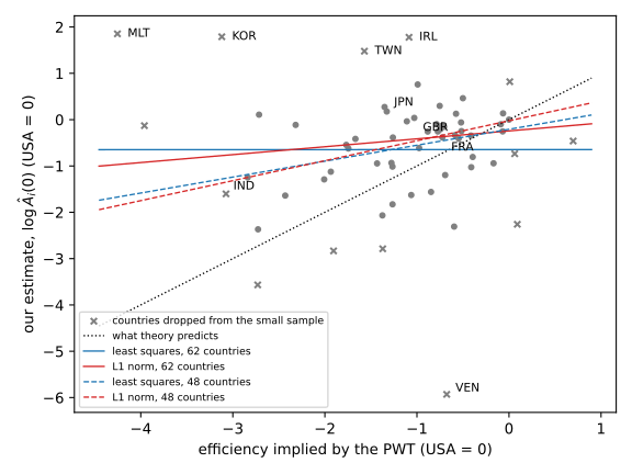
What should one retain from these three readings? Not that there is no relation — the robust fit does find one — but that it is weak, very imprecise, and three times too flat for the theory, which requires a slope of one. It would therefore be dishonest to present this estimate of the level as an achievement of the panel. What the panel identifies well is the dynamics: the speed at which countries rejoin their path. The level \(\log A_i(0)\) is a nuisance parameter that absorbs everything the model cannot explain — the absence of human capital, measurement error in initial income, the distance to the steady state in 1963 — and nothing guarantees that the sum of these residuals looks like an efficiency. The encouraging sign is that it correlates at +0.44 with human capital, which makes sense since our model contains none and \(A\) must absorb it. This also tempers the verdict the next section will draw from those same unknowns: their correlation with the saving rate does refute the orthogonality assumption, but it says nothing about the value of \(\log A_i(0)\) as a measure.
Back to the cross-section
We can now return to the questions that the cross-section note had to leave open. There were three of them, and each came from the fact that a single observation per country does not allow labour efficiency to be separated from the rest.
- Does initial income contain labour efficiency? If so, the cross-section estimator is biased. The simulations of the previous note bracketed the observed estimate, \(\hat\theta = 0.102\), between two extreme worlds — initial income without efficiency (all estimates above 0.17), initial income containing all of it (all below 0.09) — and nothing told us where the data stood.
- Is labour efficiency independent of the saving rate? Mankiw, Romer and Weil assume so, and the cross-section could only grant it.
- Is the rejection of the Solow model real? It might have been a mere effect of endogeneity, and it rested moreover on a \(\chi^2\) distribution whose actual size was 8% rather than 5%.
Let us start with the second, the easiest, for the panel answers it without simulating anything and without estimating anything more. The initial efficiency of each country is now a number: it is enough to look at whether it goes together with the saving rate. The Mankiw, Romer and Weil assumption says there is no relation at all, so that a non-zero correlation suffices to refute it.
ls, lc = np.log(S.mean(axis=0)), np.log(cbar)
draws = np.random.default_rng(8)

def association(v, x):
    """Pearson and Spearman correlations, and a resampling interval."""
    r, p = stats.pearsonr(v, x)
    bs = [np.corrcoef(v[i], x[i])[0, 1] for i in (draws.integers(0, N, N) for _ in range(2000))]
    return round(r, 3), round(p, 5), round(stats.spearmanr(v, x).statistic, 3), \
        np.percentile(bs, [2.5, 97.5]).round(3)

def partial(v, x, z):
    """Correlation of v and x once the part explained by z is removed from each."""
    Z = np.column_stack([np.ones(N), z])
    rest = lambda u: u - Z @ np.linalg.lstsq(Z, u, rcond=None)[0]
    return round(np.corrcoef(rest(v), rest(x))[0, 1], 3)

print(association(lA0_ml, ls), association(lA0_ml, lc))
print(association(lA0, ls), association(lA0, lc))   # with the within estimator's unknowns
print(round(np.corrcoef(ls, lc)[0, 1], 3),          # the two variables are themselves related
      partial(lA0_ml, ls, lc), partial(lA0_ml, lc, ls))
There is one, and it is solid.
| correlation | of ranks | partial | |
|---|---|---|---|
| \(\log\bar s_i\) | +0.35 | +0.42 | +0.29 |
| \(\log\bar c_i\) | −0.21 | −0.29 | −0.08 |
The first column is the usual correlation, Pearson's. The second is computed on ranks rather than on values, and its merit is to be insensitive to a few extreme countries: it confirms the first. The third is the partial correlation, the one that remains between two variables once the part explained by the third has been removed from each: it is useful here because the saving rate and \(\bar c_i\) are themselves correlated, at −0.40, so that either could show up merely through the other.
The reading is clear. The saving rate does go with efficiency, and this association does not run through \(\bar c_i\), since it survives its removal. The apparent correlation of \(\bar c_i\), by contrast, vanishes as soon as saving is held fixed. The association with saving is sharp: its p-value is 0.0002 and its 95% confidence interval, obtained by resampling countries, runs from 0.16 to 0.52. The orthogonality assumption is therefore false in these data, and the cross-section estimate was indeed biased.
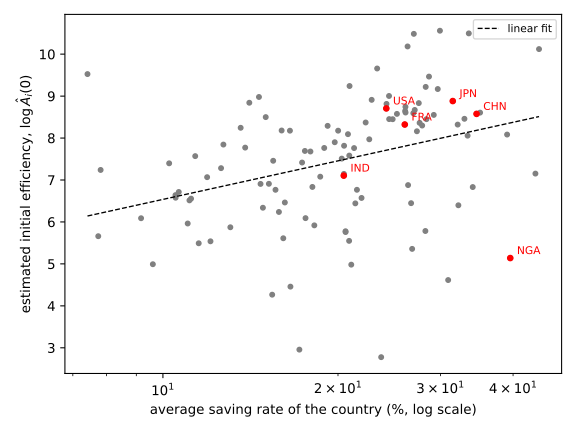
One could have regressed efficiency on the two rates, but that would have taught us nothing more: the theory does not predict a particular slope, it predicts the absence of any relation, and the value of a regression coefficient would have no structural interpretation here. The partial correlation gives the same information as a regression without suggesting one.
Two reservations about these figures. First, initial efficiency is not a datum but an estimate: the p-values and the interval above ignore that uncertainty. Second, they depend somewhat on the estimator retained: the unknowns of the within estimator give stronger correlations, +0.47 with the saving rate and −0.40 with \(\bar c_i\). The conclusion does not change.
The other two questions call for one last experiment, the most direct of the note.
def cross_section(Y):
    """M2 estimator of the cross-section note, on the incomes of 1963 and 2023."""
    t = END - START
    gy, ly0, sb = (Y[-1] - Y[0])/t, Y[0], S.mean(axis=0)
    def minus_loglik(p):
        theta, a, alpha = p
        w = (1 - np.exp(-theta*cbar*t))/t
        u = (gy - X - w*(a + alpha/(1 - alpha)*(np.log(sb) - np.log(cbar)) - ly0))/w
        return N/2*np.log(u @ u/N) + np.sum(np.log(w))
    tries = [minimize(minus_loglik, p0, method='L-BFGS-B',
                      bounds=[(1e-4, 3), (-50, 50), (0.01, 0.99)])
             for p0 in ([0.1, 7, 0.7], [0.3, 6, 0.5], [0.05, 8, 0.8], [1, 8, 0.3])]
    return min(tries, key=lambda e: e.fun).x[[0, 2]]

dice3 = np.random.default_rng(3)
in_cross_section = cross_section(LY)
world = np.array([cross_section(simulate(*star, sigma_ml, psi_ml, lA0_star, LY, S, C, K, 5, dice3))
                  for _ in range(300)])
common = np.full(N, lA0_star.mean())             # no permanent difference across countries
no_link = np.array([cross_section(simulate(*star, sigma_ml, psi_ml, common, LY, S, C, K, 5, dice3))
                    for _ in range(300)])
print(in_cross_section.round(3), np.corrcoef(lA0_ml, LY[0])[0, 1].round(2))
for name, draws in (('world', world), ('no link', no_link)):
    print(name, draws.mean(axis=0).round(3), np.percentile(draws, [5, 95], axis=0).round(3),
          np.median(draws[:, 0]).round(3), draws[:, 0].std().round(3),
          (draws[:, 0] <= in_cross_section[0]).mean().round(3))
print(np.median(np.outer([in_cross_section[0], theta5, theta_ml, star[0]], cbar), axis=1).round(4))
Applied to the years 1963 and 2023 of the panel, the estimator of the cross-section note gives \(\hat\theta = 0.105\) and \(\hat\alpha = 0.708\), roughly what it gave over 1960-2023. Now simulate the panel with the corrected parameters, \(\theta^{\star} = 0.36\) and \(\alpha^{\star} = 0.32\), the incomes observed in 1963 and the efficiencies they imply, then apply this same cross-section estimator to each simulated panel, changing nothing. It gives on average \(\hat\theta = 0.089\) and \(\hat\alpha = 0.74\), with a standard deviation of 0.022 for the former, whose central 90% interval runs from 0.057 to 0.126. The estimate obtained on the real data, 0.105, falls inside that interval, above the simulated median, 0.086. The cross-section estimate is therefore exactly what a world in which \(\theta\) equals 0.36 produces when looked at with a single observation per country.
It remains to know where the gap between 0.36 and 0.09 comes from. Let us repeat the experiment in a world that differs from the previous one in a single respect: all countries have the same initial efficiency, so that the 1963 income can no longer contain any part of it. The cross-section estimator then recovers \(\hat\theta = 0.43\) and \(\hat\alpha = 0.31\) on average, this time of the right order of magnitude, and even a little above the true value. The whole bias of the cross-section therefore comes from permanent differences in efficiency across countries and from their presence in initial income, which is quite real in the data: estimated efficiency and 1963 income have a correlation of 0.36. This is the answer to the first question: initial income contains part of labour efficiency, and that part is enough to divide by four the speed estimated in the cross-section. The previous note had diagnosed the right illness; the panel measures the dose.
The section on the measurement of labour efficiency showed that \(\log\hat A_i(0)\) is a poor measure of efficiency in the sense of growth accountants. This does not weaken the argument. What biases the cross-section is the permanent component specific to each country, whatever name one gives it, and it is precisely that component which the country unknown absorbs.
The third question receives a more nuanced answer, and it is perhaps the most important result of the two notes. The following table sets the four estimates side by side.
| Cross-section | Panel, within | Panel, ML | Panel, corrected | |
|---|---|---|---|---|
| \(\theta\) | 0.105 | 0.478 | 0.176 | 0.357 |
| \(\alpha\) | 0.708 | 0.370 | 0.508 | 0.322 |
| \(1-\alpha\) | 0.292 | 0.630 | 0.492 | 0.678 |
| median speed (% per year) | 0.86 | 3.91 | 1.44 | 2.92 |
Correcting for endogeneity moved both parameters, and in the expected direction: the speed more than tripled, and the capital share came down from 0.71 to 0.32, right at the third measured by national accounts. Endogeneity therefore explained the aberrant levels of the cross-section. It does not explain the tension between them: \(\theta^{\star}\) stays at 0.36 whereas the Solow model requires \(1-\alpha^{\star} = 0.68\), and the simulation test, which owes nothing to the \(\chi^2\), rejects the constraint. The suspicion of the previous note — that the rejection was a mere artefact — is lifted: the capital share that accounts for income differences still implies faster convergence than we observe.
These numbers also shed light on the dispersion of published estimates that the previous note surveyed. The roughly 4% per year that Islam (1995) obtains from the within estimator is what we obtain with it, and the binding function shows that it says almost nothing about the true speed. The corrected value, close to 3%, falls in the middle of the 2 to 4% range that Bond, Hoeffler and Temple (2001) obtain by an entirely different route, instruments.
The limits of the statistical model
Everything above rests on an assumption stated at the outset and never checked. It concerns the innovations \(\varepsilon_{i,k}\), and them alone: normal, independent of one another as well as across countries, and with the same variance \(\sigma^2\) everywhere. Everything else follows from it: the covariance \(\Sigma_i\) of the contrasts, hence the estimator we retained, and the null distribution of the Solow test, which is simulated from the model. If that assumption is false, this is no second-order detail.
How can we look at \(\varepsilon\), which is not observed? In two steps. The first yields the disturbance of the equation: with the estimates of the previous section, \(\hat\theta = 0.176\) and \(\hat\alpha = 0.508\), we form the residual \(r_{i,k}\), which equals \(g_{i,k}\log A_i(0) + v_{i,k+1}\), and remove from it the country unknown — the initial efficiency \(\log A_i(0)\), which we do not know — by the regression of \(r_{i,k}\) on \(g_{i,k}\):
\begin{equation*} \hat v_{i,k+1} = r_{i,k} - g_{i,k}\widehat{\log A_i(0)} \end{equation*}The second step whitens that residual, that is, undoes the moving average. The relation \(v_k = \varepsilon_k + \psi\varepsilon_{k-1}\) inverts step by step,
\begin{equation*} \hat\varepsilon_{i,k} = \hat v_{i,k} - \hat\psi\,\hat\varepsilon_{i,k-1} \end{equation*}starting from \(\hat\varepsilon_{i,1} = \hat v_{i,1}\). This gives an estimate of the innovations themselves, and it is they that we shall put to the three assumptions: no correlation from one period to the next, constant variance over time, constant variance across countries.
One precaution before reading the figures. These estimated innovations are not the true ones: the country unknown has been replaced in them by an estimate drawn from the same residuals, which correlates them mechanically, and negatively, even when the model is exact; and the whitening, which starts from an approximate initial condition, adds a distortion of its own. Comparing their autocorrelation with zero would therefore make no sense. The right benchmark is simulated rather than read off. So we manufacture 200 artificial data sets — 200 panels of 110 countries and thirteen dates, produced by the model itself — and apply to them the whole procedure: maximum likelihood estimation, residuals, whitening. The parameters used to build them are the ones we take to be closest to the truth, namely the corrected values \(\theta^{\star} = 0.36\) and \(\alpha^{\star} = 0.32\), with \(\hat\sigma = 0.20\), \(\hat\psi = 0.29\) and the estimated efficiencies: if the model is true, that is where our data come from, and the 200 panels then tell us what each statistic should be worth.
def whitened(v, psi):
    """Innovations recovered by inverting the moving average."""
    e = np.empty_like(v)
    e[0] = v[0]
    for k in range(1, v.shape[0]):
        e[k] = v[k] - psi*e[k-1]
    return e

def residuals_and_contrasts(Y):
    """Residuals, whitened innovations and contrasts, at the MLE of panel Y."""
    th, al, _, ps = mle(Y, S, C, K, 5, starts=((theta_ml, alpha_ml, omega_ml, psi_ml),))
    r, gg = raws([th, al], Y, S, C, K, 5)
    A = (gg*r).sum(axis=0)/(gg*gg).sum(axis=0)
    v, u = r - gg*A, r/gg
    return v, whitened(v, ps), u[1:] - u[:-1]

def autocorr(x, lag):
    """Empirical autocorrelation, pooled across countries."""
    return np.corrcoef(x[:-lag].ravel(), x[lag:].ravel())[0, 1]

LAGS = (1, 2, 3, 4)
v_obs, e_obs, z_obs = residuals_and_contrasts(LY)
av_obs = np.array([autocorr(v_obs, l) for l in LAGS])     # the disturbance v
ac_obs = np.array([autocorr(e_obs, l) for l in LAGS])     # the innovations
zc_obs = np.array([autocorr(z_obs, l) for l in (1, 2)])
sp = e_obs.std(axis=0)

draw = np.random.default_rng(7)
AV, AC, ZC, SDP, RATIO = [], [], [], [], []
for _ in range(200):
    Y = simulate(*star, sigma_ml, psi_ml, lA0_star, LY, S, C, K, 5, draw)
    v, e, z = residuals_and_contrasts(Y)
    AV.append([autocorr(v, l) for l in LAGS])
    AC.append([autocorr(e, l) for l in LAGS])
    ZC.append([autocorr(z, l) for l in (1, 2)])
    SDP.append(e.std(axis=1))
    RATIO.append(e.std(axis=0).max()/np.median(e.std(axis=0)))
AV, AC, ZC = np.array(AV), np.array(AC), np.array(ZC)
SDP, RATIO = np.array(SDP), np.array(RATIO)

print(ac_obs.round(3), AC.mean(axis=0).round(3),
      np.percentile(AC, [5, 95], axis=0).round(3))
print(av_obs.round(3), AV.mean(axis=0).round(3),
      np.percentile(AV, [5, 95], axis=0).round(3))
print(zc_obs.round(3), np.percentile(ZC, [5, 95], axis=0).round(3))
print(e_obs.std(axis=1).round(3), np.percentile(SDP, [5, 95]).round(3),
      sp.min().round(3), codes[sp.argmin()],
      np.median(sp).round(3), sp.max().round(3), codes[sp.argmax()])
print((sp.max()/np.median(sp)).round(2), np.percentile(RATIO, 95).round(2),
      (e_obs.mean(axis=1).var()/e_obs.var()).round(4))
The innovations remain correlated, at the third lag. At lags 1 to 4 the autocorrelation of the estimated innovations is −0.070, −0.066, −0.230 and −0.053, where the model, simulated, expects −0.098, −0.106, −0.095 and −0.086. The first lag is nearly back in order: −0.070 against a band of [−0.115; −0.083], whose bound it exceeds by only thirteen thousandths, where the disturbance \(v\) showed +0.194. That is the work of the moving average, and that is what it was asked to do. The second and fourth lags are inside their bands. The third, however, is −0.230 against [−0.149; −0.036]: there remains at that lag a dependence the moving average does not capture, and hence innovations that are not independent.
It remains to check the explanation put forward earlier, that of temporal aggregation, for nothing compelled the correlation to come from there rather than from the economics. The prediction is precise, and therefore testable. Sampling every five years a process that evolves continuously induces no correlation — innovations accumulated over disjoint intervals stay independent; averaging a flow does induce one, positive. So let us simulate the model at annual frequency, then rebuild the five-year panel in both ways, by point sampling and by period averaging, and compare.
n_yr = pop_yr[1:]/pop_yr[:-1] - 1
c_yr = np.clip(n_yr + X + delta_yr[:-1], 1e-3, None)
s_pos = np.clip(s_yr[:-1], 1e-3, None)
rho_yr, a2 = np.exp(-theta_ml*c_yr), alpha_ml/(1 - alpha_ml)

def annual(u):
    """Annual trajectory of the same model, without aggregation, for a given shock u."""
    Y = np.empty((END - START + 1, N))
    Y[0] = ly_yr[0]
    for t in range(END - START):
        Y[t+1] = (rho_yr[t]*Y[t] + (1 - rho_yr[t])*(a2*(np.log(s_pos[t]) - np.log(c_yr[t]))
                  + lA0_ml) + X*(1 + t*(1 - rho_yr[t])) + u[t])
    return Y

def on_grid(Yan, averaged, tau=5):
    """Grid of step tau: point sampling, or average around the date."""
    d, half = np.arange(0, END - START + 1, tau), tau//2
    if not averaged:
        return Yan[d, :]
    return np.array([Yan[max(k-half, 0):k+half+1, :].mean(axis=0) for k in d])

for averaged in (False, True):
    dice, AG = np.random.default_rng(11), []
    for _ in range(60):
        # 0.10: annual standard deviation which, aggregated, matches the observed noise
        noise = dice.normal(0, 0.10, (END - START, N))
        e, _, _ = residuals_and_contrasts(on_grid(annual(noise), averaged))
        AG.append([autocorr(e, l) for l in LAGS])
    print(averaged, np.mean(AG, axis=0).round(3))
The verdict is clear. Rebuilt by point sampling, the model produces no positive correlation; rebuilt from period averages, it produces one at the first lag and deepens the following ones, that is, exactly the observed signature. Temporal aggregation therefore explains not only the sign but the shape.
The prediction can be checked a second time, independently. If \(\psi\) really comes from the period average, it must fade as the periods lengthen, since an averaged year then weighs less. So let us redo the estimation on the same sample split into six ten-year periods, and trace the profile of the criterion around the optimum to see whether the \(\psi\) found is identified or merely indeterminate.
LY10, S10, C10, K10 = panel(10)            # the same sample, in six periods
psi10 = mle(LY10, S10, C10, K10, 10)[3]
profile = {psi: minimize(lambda q: loglik([q[0], q[1], q[2], np.arctanh(psi/0.95)],
                                          LY10, S10, C10, K10, 10),
                         start(0.2, 0.55)[:3], method='Nelder-Mead').fun
           for psi in (-0.2, -0.1, 0.02, 0.1, 0.2)}
trough = min(profile.values())
print(round(psi10, 3), {k: round(v - trough, 1) for k, v in profile.items()})
\(\hat\psi\) falls to 0.02, and the profile shows that this zero is well determined: imposing \(\psi = -0.1\) costs 1.6 points of log-likelihood, \(\psi = +0.1\) costs 0.8, and \(\psi = \pm0.2\) more than four. The parameter \(\psi\) therefore measures a convention of measurement, not an economic mechanism.
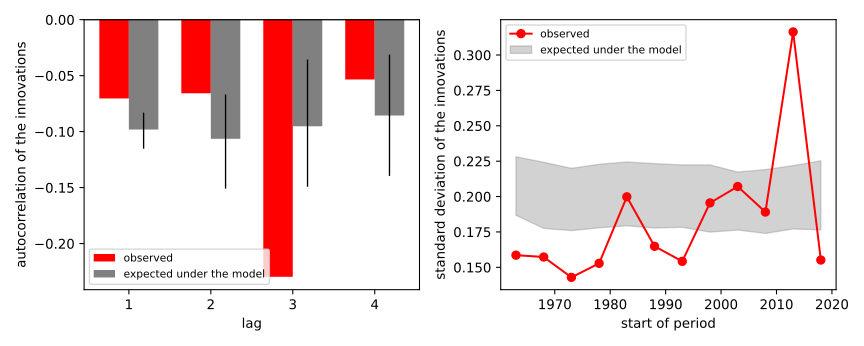
Should the error process then be enriched? The question arises, and it can be estimated: it is enough to allow moving-average coefficients at other lags, which the covariance \(V\) accepts without a single change elsewhere.
def ml_lags(lags):
    """Maximum likelihood with moving-average coefficients at the given lags."""
    def minus_l(x):
        psis = np.zeros(max(lags))
        psis[np.array(lags) - 1] = 0.95*np.tanh(x[3:])
        return criterion(np.exp(x[0]), 0.01 + 0.98/(1 + np.exp(-x[1])), np.exp(x[2]),
                         psis, LY, S, C, K, 5)
    a = (0.508 - 0.01)/0.98
    x0 = np.array([np.log(0.176), np.log(a/(1 - a)), np.log(1.272)]
                  + [np.arctanh(0.29/0.95)]*len(lags))
    tries = [minimize(minus_l, x0 + d, method='Nelder-Mead',
                      options=dict(maxiter=8000, xatol=1e-7, fatol=1e-9)) for d in (0.0, 0.1)]
    x = min(tries, key=lambda e: e.fun).x
    return (-min(tries, key=lambda e: e.fun).fun, np.exp(x[0]),
            0.01 + 0.98/(1 + np.exp(-x[1])), (0.95*np.tanh(x[3:])).round(3))

for lags in ([1], [1, 2, 3], [1, 3]):
    l, th, al, ps = ml_lags(lags)
    print(lags, round(l, 2), round(th, 4), round(al, 4), ps)
| errors | log-likelihood | \(\hat\theta\) | \(\hat\alpha\) | coefficients |
|---|---|---|---|---|
| MA(1) | 2042.27 | 0.176 | 0.508 | \(\psi_1 = 0.294\) |
| MA(3) | 2050.19 | 0.179 | 0.516 | 0.299; 0.004; −0.123 |
| MA at lags 1 and 3 | 2050.18 | 0.179 | 0.516 | 0.297; −0.125 |
Three lessons. First, the third lag is indeed real: gaining it is worth 15.8 points of likelihood ratio for a single parameter, which no accident produces. Second, the second lag is useless: the full MA(3) and its version constrained to \(\psi_2 = 0\) reach the same likelihood, to within a hundredth, the latter with one parameter fewer. The specification the data prefer is therefore \(v_{i,k} = \varepsilon_{i,k} + \psi_1\varepsilon_{i,k-1} + \psi_3\varepsilon_{i,k-3}\), with \(\hat\psi_1 = 0.297\) and \(\hat\psi_3 = -0.125\). Third, and this is what matters for this note, the parameter of interest does not move: 0.176 with the MA(1), 0.179 with the extra lag, that is a twelfth of the standard error of \(\hat\theta\). We therefore keep the MA(1) as the reference — flow aggregation justifies it, it is more parsimonious, and the conclusions of the note do not depend on it — but one should know that the data reject it.
Where can a dependence three periods apart come from? We do not know. Three five-year periods make fifteen years, and we can see no mechanism, economic or measurement-related, that would produce a correlation at that horizon and at that one alone. We therefore leave the fact as it stands: it is a reservation about the statistical model, not a result of the note — and, as the table above shows, the speed of convergence does not depend on it.
The variance is not constant over time. The standard deviation of the estimated innovations goes from 0.143 over the period starting in 1973 to 0.316 over the one starting in 2013, where the simulated band runs from 0.178 to 0.223, and period means account for 8.0% of their variance. The model predicts nothing of the sort, since its trend \(\gamma_{i,k}\) is common but deterministic. This is a serious argument for the time dummies that the section From cross-section to panel dismissed rather too quickly: they cost \(K-1\) parameters, but they absorb these common shocks, and the comparison of fit in the section on the within estimator shows that they more than pay for themselves, since they double the explained share of growth.
Nor is it constant across countries. The standard deviation of the innovations ranges from 5.0% in Australia to 95.9% in Venezuela, for a median of 13.5%. The ratio of the maximum to the median is 7.1, whereas the model makes it exceed 1.8 in only 5% of samples. A single \(\sigma\) for 110 countries is a convenient fiction.
The figure hints at a regularity, and it holds up: rich economies are the calmest. The correlation between \(\log\hat\sigma_i\) and the country's average income per head, also in logarithm, is −0.27, a t-ratio of −2.9, and it survives dropping the five most turbulent countries. The slope is −0.12: doubling income per head lowers the standard deviation of the innovations by 8%. It is not, however, a smooth gradient. The medians of \(\hat\sigma_i\) by income quartile are 14.7%, 15.0%, 15.2% and 8.6%: the first three quarters are indistinguishable and only the richest stands apart, so that the level of development accounts for no more than 7% of the dispersion. We have no more of an explanation to offer here than in the previous paragraph — diversification of output, macroeconomic stabilisation, quality of the national accounts are all plausible, and none is tested in this note.
level = LY.mean(axis=0)                   # the country's average income per head, in logarithm
income_slope, intercept = np.polyfit(level, np.log(sp), 1)
quartile = np.digitize(level, np.quantile(level, [0.25, 0.5, 0.75]))
resid = np.log(sp) - (intercept + income_slope*level)
print(round(np.corrcoef(level, np.log(sp))[0, 1], 3), round(income_slope, 3),
      round(1 - resid.var()/np.log(sp).var(), 3),
      [round(100*float(np.median(sp[quartile == j])), 1) for j in range(4)])
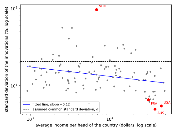
One objection remains, and it must be examined because it seems to absolve everything. The likelihood does not bear on the innovations, but on the contrasts
\begin{equation*} z_{i,k} = u_{i,k} - u_{i,k-1} = \frac{v_{i,k+1}}{g_{i,k}} - \frac{v_{i,k}}{g_{i,k-1}} \end{equation*}to which it assigns the covariance \(\sigma^2\Sigma_i = \sigma^2 T_i V T_i'\). So let us check that object rather than the innovations: its correlation is −0.49 at the first lag and −0.01 at the second, and both fall inside the simulated bands, [−0.50; −0.32] and [−0.19; 0.00]. What the estimator looks at is therefore consistent with the data.
It would be tempting to read this as a refutation of everything above. That would be a misreading, for two reasons. The first is that the check has little power: differencing alone imposes a correlation close to −0.5 at the first lag, and the bands are wide. The second is more fundamental. Everything in these contrasts comes from the innovations:
\begin{equation*} z_i = T_i r_i,\qquad r_i = g_i\log A_i(0) + M\varepsilon_i \end{equation*}where \(M\) is the moving-average matrix, the one satisfying \(V = MM'\). Since \(T_i\) removes \(\log A_i(0)\) from every component but the first, the contrasts are, that one aside, a linear function of the \(\varepsilon_{i,k}\) alone. The assumptions therefore bear, in the last resort, on \(\varepsilon\) and on it alone: if \(\varepsilon\) violates them, so does \(z\). A check on \(z\) that detects nothing does not clear \(\varepsilon\); it only says that the transformation — differencing, dividing by \(g_{i,k}\), pooling countries with very unequal standard deviations — has diluted the trace to the point of making it undetectable.
The right question therefore lies elsewhere: what becomes of the estimator when the distribution assumed for \(\varepsilon\) is wrong, while the equation giving its mean remains correct? The likelihood ceases to be the true likelihood and is no more than one criterion among others — one speaks of a pseudo-likelihood. It still has a maximum, but the binding function used to correct the bias and the variance used to test are both computed under a distribution that is not the one the data come from.
What should one conclude for the results of this note? The correction by indirect inference keeps its meaning: it assumes nothing beyond the model's ability to reproduce an auxiliary statistic, and would merely be less efficient if the distribution of the errors is misspecified. The Solow test is more exposed, since its null distribution is simulated with these same misspecified errors. Its verdict is probably still right — the observed gap, −0.32, is more than four times the bound of the simulated band, ±0.07, and it would take an enormous specification error to bridge such a chasm — but "probably" is the right word here, and a robust version of the test remains to be written. The three natural remedies are a country-specific \(\sigma_i\), common time effects, and a variance robust to misspecification, the so-called sandwich, for inference; none is free, and each would deserve a note of its own.
Entirely free speeds
Before concluding, one last point of comparison, which places the structural restriction against the other extreme. Everything above imposes on country \(i\) the speed \(\theta\,c_{i,k}\); one may instead impose nothing at all and estimate one speed per country, on annual data.
def free_speeds(trend):
    """One regression per country on annual data, and the implied speed."""
    rho = np.empty(N)
    for i in range(N):
        cols = [np.ones(END - START), ly_yr[:-1, i]]
        if trend:
            cols.append(np.arange(END - START))
        rho[i] = np.linalg.lstsq(np.column_stack(cols), ly_yr[1:, i], rcond=None)[0][1]
    return rho

free = {}
for trend in (False, True):
    rho = free_speeds(trend)
    ok = rho < 1
    beta = -np.log(np.clip(rho, 1e-6, None))
    free[trend] = (beta, ok)
    A = np.column_stack([np.ones(ok.sum()), cbar[ok]])
    co = np.linalg.lstsq(A, beta[ok], rcond=None)[0]
    res = beta[ok] - A @ co
    V = np.linalg.inv(A.T @ A)*(res @ res)/(ok.sum() - 2)
    print(trend, (~ok).sum(), np.median(beta[ok]).round(4), beta[ok].mean().round(4),
          beta[ok].std().round(4), co[1].round(3), np.sqrt(V[1, 1]).round(3))
The result is a warning. Without a trend, 26 countries out of 110 have a \(\hat\rho_i\) greater than or equal to one, that is, do not converge at all; for the others, the median speed is 2.7% per year, the mean 5.0% and the standard deviation 5.8 points. Regressing these speeds on \(\bar c_i\), which the model would want to have slope \(\theta\), gives 0.45 with a standard error of 0.41: the structural prediction is neither confirmed nor refuted, the free estimate being too imprecise to decide. And everything flips if a trend is added to each regression: only 3 countries fail to converge, the median speed rises to 8.4% and the slope falls to 0.14 with a standard error of 0.55. Lee, Pesaran and Smith (1997) ran the same experiment and went further: leaving both the level and the trend free, country by country, they obtain a speed of the order of 30% per year, which they themselves judge very imprecise and hard to interpret. The direction is the same as ours: the more parameters are freed per country, the higher the estimated speed, and the less precise.
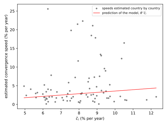
One can measure here what the structural restriction buys. Arnold, Bassanini and Scarpetta (2011) start from the same observation as this note — the model implies speeds that differ across countries — but draw the opposite conclusion: they estimate one free speed per country, and use \(n_i+x+\delta_i\) as a mere control variable. The structural relation is then a motivation, never a constraint. Imposing it costs an assumption and buys two things: estimable speeds, and a test.
Conclusion
The panel delivers most of what it promised. The cross-section note ended on a doubt it could not lift: did its rejection of the Solow model come from the model, or from the endogeneity of initial income? The answer is now twofold. Endogeneity is real and measurable: the labour efficiency recovered from the country unknowns increases with the saving rate, which refutes the Mankiw, Romer and Weil assumption, and it is correlated with initial income, which is enough to divide by four the speed estimated in the cross-section — panels simulated with the corrected speed give back, seen as a cross-section, the estimate of the previous note. But the rejection of the Solow model was not an artefact of it: once endogeneity is removed, the capital share falls to 0.32 and the speed rises to 2.9% per year, without the one meeting the other.
Getting there took more than a change of data. The panel introduces a problem the cross-section did not have, and one whose severity is understated by reciting Nickell's order of magnitude: at the noise level of these data, the within estimator is nearly mute on the speed of convergence. Indirect inference gets around it, provided one inverts an estimator that responds to the parameter, even a biased one. The resulting verdict no longer rests on an exogeneity assumption nor on an asymptotic approximation. It does rest, however, on the distribution ascribed to the disturbances. Those disturbances are correlated from one period to the next, the section on the limits shows that the cause lies in how the data are dated rather than in any economic mechanism, and the model takes it into account. What it does not correct is heteroskedasticity: the standard deviation of the disturbances varies by a factor of more than twenty from one country to another, and the rejection of Solow, wide though it is, has not been tested against that particular misspecification. It finally remains to submit the model to instruments, which will be the subject of a forthcoming note.
Exercises
Establish that \(\gamma_{i,k} = x\bigl[\tau + t_k\,g_{i,k}\bigr]\). What does one assume by replacing it with a dummy per period, as is customary?
Solution
Writing \(\log y_{i,k} = \log A_i(0) + xt_k + \log\hat y_{i,k}\) and substituting into the dynamics of \(\log\hat y\), the term in \(x\) that remains on the right hand side is \(xt_{k+1} - \rho_{i,k} xt_k\). Since \(t_{k+1} = t_k+\tau\), it equals \(x\tau + xt_k(1-\rho_{i,k})\). It therefore depends on the country and on the period, through \(\rho_{i,k}\), and grows with the date. A dummy per period, by contrast, imposes the same term on every country: it absorbs common shocks, which is often desirable, but also part of the structural dynamics, and it consumes \(K-1\) parameters that the model provided for free.
Show that the regression of \(r_{i,k}\) on \(g_{i,k}\) reduces to the time average of the residuals when the rates are constant. Check numerically that the two expressions then give the same estimate, and measure the gap when the rates vary.
Solution
If \(g_{i,k} = g_i\) does not depend on \(k\), then \(\sum_k g_i r_{i,k}/\sum_k g_i^2 = \bar r_i/g_i\), and the concentrated residual \(r_{i,k} - g_i\bar r_i/g_i = r_{i,k} - \bar r_i\) is exactly that of the within transformation.
def within_naive(LY, S, C, K, tau):
    """Faulty variant: simple average of the residuals, ignoring the coefficient g."""
    def criterion(p):
        r, _ = raws(p, LY, S, C, K, tau)
        return (r - r.mean(axis=0)).ravel()
    return min([least_squares(criterion, p0, bounds=([1e-4, 0.01], [5, 0.99]))
                for p0 in ([0.4, 0.4], [0.1, 0.7], [0.03, 0.5])], key=lambda e: e.cost)

Cfixed = np.tile(C.mean(axis=0), (K, 1))
print(within(LY, S, Cfixed, K, 5).x.round(4), within_naive(LY, S, Cfixed, K, 5).x.round(4))
print(within(LY, S, C, K, 5).x.round(4), within_naive(LY, S, C, K, 5).x.round(4))
With the rates frozen at their average, the two estimators agree to four decimals. With period-specific rates, the version that ignores \(g_{i,k}\) collapses to 0.07 against 0.48: it does not eliminate the country unknown, and the gap is not a numerical detail but a specification error.
The likelihood of the section on maximum likelihood carries the term \(\sum_{k\geq2}\log g_{i,k}\). Where does it come from, and what happens without it? Check that it reduces to a constant when the rates are held fixed.
Solution
It is the Jacobian of the change of variables. The likelihood is written for the transformed vector \(z\), whereas the data are the residuals \(r\); the density of the former is that of the latter divided by the absolute determinant of the transformation, here \(\prod_{k\geq2} 1/g_{i,k}\). Since the \(g\) depend on \(\theta\), the term does not vanish into a constant and must be carried. Dropping it hands the optimiser a free way of improving the criterion: inflating the \(g\) raises the determinant without explaining anything, and \(\theta\) runs to its upper bound. When the rates are constant, \(g_{i,k} = g_i\) and the term becomes \((K-1)\sum_i\log g_i\), which is exactly compensated by the change in the determinant of \(\Sigma_i\); the two writings then give the same estimate.
Compute the order of magnitude of the Nickell bias, \(-(1+\rho)/(K-1)\), for \(\rho = 0.84\) and \(K = 12\), then translate it into a convergence speed. Compare with the Monte Carlo of the section on the bias of the within estimator.
Solution
The bias equals \(-1.84/11 \simeq -0.17\), that is \(\hat\rho \simeq 0.67\) instead of 0.84, and a speed of \(-\log(0.67)/5 = 8.0\%\) per year instead of 3.4%. The direction is right, but the Monte Carlo shows the analogy to be misleading: in the linear model the bias is a translation one can subtract, whereas here the function relating the true parameter to the expectation of its estimator is flat over a whole range. It is not the same disease, and it is not cured in the same way.
A panel can grow in two directions: by adding countries or by adding periods. Simulate panels of increasing size in each of them, replicating the observed rates and efficiencies, and apply both estimators to them. In which direction does the bias fade, and why? What follows for our data?
Solution
enlarge, TRUE = np.random.default_rng(19), 0.176   # as in the binding function

def enlarged(m, q):
    """Panel simulated with m copies of the countries and q copies of the periods."""
    Sg, Cg, lA0g = np.tile(S, (q, m)), np.tile(C, (q, m)), np.tile(lA0_ml, m)
    Kg, mould = q*K, np.empty((q*K + 1, m*N))
    mould[0] = np.tile(LY[0], m)
    Y = simulate(TRUE, 0.508, sigma_ml, psi_ml, lA0g, mould, Sg, Cg, Kg, 5, enlarge)
    return Y, Sg, Cg, Kg

for m, q in ((1, 1), (2, 1), (8, 1), (1, 2), (1, 4), (1, 8)):
    W, M = [], []
    for _ in range(15):
        Y, Sg, Cg, Kg = enlarged(m, q)
        W.append(within(Y, Sg, Cg, Kg, 5).x[0])
        M.append(mle(Y, Sg, Cg, Kg, 5, starts=((TRUE, 0.508, omega_ml, psi_ml),))[0])
    print(110*m, Kg, round(np.mean(W), 3), round(np.std(W), 3),
          round(np.mean(M), 3), round(np.std(M), 3))
The table gives the average of the estimates and, in parentheses, their standard deviation, for a true \(\theta\) of 0.176 and the nuisance parameters of the correction, the maximum likelihood efficiencies included. The ML column is therefore comparable with the binding function of the main text; the within column is not, the bias table having been simulated, for want of anything better, with the within efficiencies.
| countries | periods | within | ML |
|---|---|---|---|
| 110 | 12 | 0.365 (0.038) | 0.112 (0.028) |
| 220 | 12 | 0.388 (0.040) | 0.107 (0.024) |
| 880 | 12 | 0.384 (0.012) | 0.106 (0.010) |
| 110 | 24 | 0.258 (0.018) | 0.160 (0.033) |
| 110 | 48 | 0.190 (0.013) | 0.175 (0.019) |
| 110 | 96 | 0.155 (0.005) | 0.173 (0.007) |
Multiplying countries fixes nothing. From 110 to 880 countries the estimates tighten — the standard deviation is divided by three — but around a wrong value: 0.384 for the within estimator and 0.106 for maximum likelihood, when the truth is 0.176. This is what incidental parameters do: each additional country brings twelve observations and one more unknown, so that \(\log A_i(0)\) is never estimated any better. And that is the direction in which our data look most like a large sample.
Lengthening the span works, for maximum likelihood. At a given number of countries, its estimate goes from 0.112 to 0.160, then 0.175 and 0.173, and its standard deviation falls from 0.028 to 0.007. The within estimator, by contrast, goes down from 0.365 to 0.155, crossing the true value on its way: it ignores the correlation of the errors, which is a misspecification from its point of view, and a misspecification does not fade away as the sample grows.
Two cautions in reading this. Seeing a distribution tighten on a grid of sample sizes is not a proof of convergence in probability, and an average that gets closer would not suffice — the dispersion must also vanish, which the standard deviation allows one to monitor. And both experiments are artificial, since they manufacture data we do not have. The practical conclusion is no less clear: with twelve periods, the bias must be corrected rather than hoped away.
Suppose each country follows a random walk with drift, \(y_{i,t} = y_{i,t-1} + \mu + \varepsilon_{i,t}\), the \(\varepsilon\) being independent, with zero mean and variance \(\sigma^2\). There is therefore no convergence at all. Show that the within slope tends, as the number of countries grows, to
\begin{equation*} 1 - \frac{3\sigma^2}{(T+1)\left(\sigma^2 + \mu^2 T/2\right)} \end{equation*}where \(T\) is the number of transitions. What is this limit without drift? What does it become as \(T\) grows? Check it by simulation.
Solution
Write \(x_{i,t} = y_{i,t-1}\) for the regressor and \(\tilde x\) for its deviation from the country average. Since \(y_t = x_t + \mu + \varepsilon_t\) and the constant disappears with the centring,
\begin{equation*} \hat\rho - 1 = \frac{\sum_i\sum_t \tilde x_{i,t}\,\tilde\varepsilon_{i,t}}{\sum_i\sum_t \tilde x_{i,t}^2} \end{equation*}Divide top and bottom by the number of countries. Each sum becomes an average of independent, identically distributed terms, one per country. Those terms are quadratic forms in shocks of finite variance, hence have a finite expectation: the law of large numbers applies separately to the numerator and to the denominator, and each converges in probability to the expectation of one term. The latter limit being strictly positive, Slutsky's lemma licenses the passage to the ratio.
Two precautions about that step. First, for an independent and identically distributed sequence, the existence of the expectation is enough for the law of large numbers. The elementary proof, through Chebyshev's inequality — the variance of an average of \(N\) independent terms is that of one term divided by \(N\), and so tends to zero — is perfectly valid, but it additionally requires shocks with a finite fourth moment, which the statement does not assume. Second, this really is a limit in probability as the number of countries grows, at fixed \(T\), and not the expectation of \(\hat\rho\), which is not the ratio of the expectations.
The numerator. We have \(\sum_t \tilde x_t\tilde\varepsilon_t = \sum_t x_t\varepsilon_t - T\bar x\bar\varepsilon\). The first term has zero mean, since \(x_t\) depends only on shocks prior to \(t\). The second does not, and that is the whole problem: the average \(\bar x\) contains the shocks, with \(\mathbb{E}[\bar x\bar\varepsilon] = \sigma^2(T-1)/(2T)\), so that
\begin{equation*} \mathbb{E}\Bigl[\sum_t \tilde x_t\tilde\varepsilon_t\Bigr] = -\frac{\sigma^2(T-1)}{2} \end{equation*}Subtracting the country average means subtracting a quantity that contains future shocks: the transformed regressor and the transformed error become correlated, negatively.
The denominator. Drift and shocks contribute to it separately. For the random part, \(\mathbb{E}[x_tx_s] = \sigma^2\min(t-1,s-1)\) and \(\sum_{a,b=0}^{T-1}\min(a,b) = (T-1)T(2T-1)/6\), whence a contribution of \(\sigma^2(T^2-1)/6\). For the drift, \(x_t\) contains \(\mu(t-1)\), whose deviations from the average have sum of squares \(\mu^2T(T^2-1)/12\). The ratio of the two limits gives the announced formula.
The two cases. Without drift it reduces to \(1 - 3/(T+1)\), that is 0.769 for our twelve transitions: a considerable bias. With drift the denominator grows and the bias melts away. And as \(T\) grows the limit tends to one in both cases, at rate \(1/T\): this is again the lesson of the previous exercise, lengthening the span helps, multiplying countries does not.
mu_rw, sig_rw = dy.mean(), (dy - dy.mean(axis=0)).std()
limit = lambda mu, sig: 1 - 3*sig**2/((K + 1)*(sig**2 + mu**2*K/2))
print(round(mu_rw, 4), round(sig_rw, 4), round(limit(0, sig_rw), 4), round(limit(mu_rw, sig_rw), 4))

attempt = np.random.default_rng(5)
for drift in (0.0, mu_rw):
    P = []
    for _ in range(400):
        Y = np.vstack([np.zeros(N), np.cumsum(drift + attempt.normal(0, sig_rw, (K, N)), axis=0)])
        bf, af = Y[:-1, :], Y[1:, :]
        P.append(slope(bf - bf.mean(axis=0), af - af.mean(axis=0)))
    print(round(drift, 4), round(float(np.mean(P)), 4))
On our data the drift is 0.1025 per five-year period and the standard deviation of the shocks 0.2074. The formula then gives 0.9064, and four hundred simulated panels give 0.9063 — the slope observed on the real data being 0.906. Without drift, the formula gives 0.769 and the simulation 0.7691. The bias of the within estimator in a world without convergence is therefore no numerical mystery: it can be written down.
References
The orthogonality assumption discussed here is that of Mankiw, N. G., Romer, D. and Weil, D. (1992), "A Contribution to the Empirics of Economic Growth", Quarterly Journal of Economics, 107(2), 407-437. The framework of this note is that of Islam, N. (1995), "Growth Empirics: A Panel Data Approach", Quarterly Journal of Economics, 110(4), 1127-1170, who first treated the convergence regression as a dynamic panel. On the bias of the within estimator, see Nickell, S. (1981), "Biases in Dynamic Models with Fixed Effects", Econometrica, 49(6), 1417-1426, and, for its analytical correction, Kiviet, J. (1995), "On Bias, Inconsistency and Efficiency of Various Estimators in Dynamic Panel Data Models", Journal of Econometrics, 68(1), 53-78. The likelihood in differences is that of Hsiao, C., Pesaran, M. H. and Tahmiscioglu, A. K. (2002), "Maximum Likelihood Estimation of Fixed Effects Dynamic Panel Data Models Covering Short Time Periods", Journal of Econometrics, 109(1), 107-150. Indirect inference is due to Gouriéroux, C., Monfort, A. and Renault, E. (1993), "Indirect Inference", Journal of Applied Econometrics, 8(S1), S85-S118, and its application to dynamic panels to Gouriéroux, C., Phillips, P. C. B. and Yu, J. (2010), "Indirect Inference for Dynamic Panel Models", Journal of Econometrics, 157(1), 68-77.
On heterogeneous speeds, see Lee, K., Pesaran, M. H. and Smith, R. (1997), "Growth and Convergence in a Multi-Country Empirical Stochastic Solow Model", Journal of Applied Econometrics, 12(4), 357-392, and Pesaran, M. H. and Smith, R. (1995), "Estimating Long-Run Relationships from Dynamic Heterogeneous Panels", Journal of Econometrics, 68(1), 79-113. The comparison at the end of the note is with Arnold, J., Bassanini, A. and Scarpetta, S. (2011), "Solow or Lucas? Testing Speed of Convergence on a Panel of OECD Countries", Research in Economics, 65(2), 110-123. An entirely different route, which bypasses fixed effects by going through the dynamics of the capital-output ratio, is that of McQuinn, K. and Whelan, K. (2007), "Conditional Convergence and the Dynamics of the Capital-Output Ratio", Journal of Economic Growth, 12(2), 159-184. The quasi-differencing of panels with varying coefficients is that of Holtz-Eakin, D., Newey, W. and Rosen, H. (1988), "Estimating Vector Autoregressions with Panel Data", Econometrica, 56(6), 1371-1395. The instrumental-variable estimates cited in the return to the cross-section are those of Bond, S., Hoeffler, A. and Temple, J. (2001), "GMM Estimation of Empirical Growth Models", CEPR Discussion Paper 3048. The correlation induced by temporal aggregation is established by Working, H. (1960), "Note on the Correlation of First Differences of Averages in a Random Chain", Econometrica, 28(4), 916-918.
The data come from version 11.0 of the Penn World Tables (Groningen Growth and Development Centre, 2025, doi:10.34894/FABVLR), described in Feenstra, R., Inklaar, R. and Timmer, M. (2015), "The Next Generation of the Penn World Table", American Economic Review, 105(10), 3150-3182.