To estimate the Solow model, Mankiw, Romer and Weil (1992) assume that every economy converges to its balanced growth path at the same speed. The model says otherwise: the convergence speed, \((1-\alpha)(n+x+\delta)\), depends on population growth and on the depreciation rate, which differ across countries. This note estimates the model by maximum likelihood, which exploits the form of heteroskedasticity the model implies, with a common capital share and a country-specific speed, on the Penn World Tables (110 countries, 1960-2023). Country-specific speeds barely improve the fit, and the full Solow model is rejected: the capital share that accounts for income differences implies convergence three times faster than the one we estimate. A simulation shows, however, that this rejection may come from an endogeneity bias that a cross-section cannot remove. Computations are done in Python, and the solutions to the exercises are given in collapsible blocks.
The Mankiw, Romer and Weil regression
We take the Solow model with a Cobb-Douglas production function, in the notation of the note on simulating the Solow model: \(s\) is the saving rate, \(n\) the growth rate of population, \(x\) that of labour efficiency \(A\), \(\delta\) the depreciation rate and \(\alpha\) the elasticity of output with respect to capital. In the neighbourhood of the balanced growth path, the gap between output per efficiency unit of labour, \(\hat y = y/A\), and its steady-state value shrinks at the rate \(\beta = (1-\alpha)(n+x+\delta)\), the convergence speed: \(\log\hat y(t) - \log\hat y^{\star} \approx e^{-\beta t}\bigl(\log\hat y(0) - \log\hat y^{\star}\bigr)\). Going back to income per head \(y\), with \(A(t) = A(0)e^{xt}\), the average annual growth rate between dates \(0\) and \(t\) is
\begin{equation*} \bar g_{y}(0,t) \equiv \frac{\log y(t) - \log y(0)}{t} = x + \frac{1-e^{-\beta t}}{t}\Bigl(\log\hat y^{\star} + \log A(0) - \log y(0)\Bigr) \end{equation*}where \(\log\hat y^{\star} = \frac{\alpha}{1-\alpha}\bigl(\log s - \log(n+x+\delta)\bigr)\). Initial labour efficiency is not observed: for country \(i\), we write \(\log A_i(0) = a + \varepsilon_i\), where \(\varepsilon_i\) is a disturbance with zero mean.
If the convergence speed is the same in every country, the factor \((1-e^{-\beta t})/t\) is a constant and the growth equation is linear:
\begin{equation*} \bar g_{y,i} = a_0 + a_1\log y_i(0) + a_2\log s_i + a_3\log(n_i+x+\delta) + u_i \end{equation*}with \(a_1 = -(1-e^{-\beta t})/t\), \(a_2 = -a_1\alpha/(1-\alpha)\), \(a_3 = -a_2\) and \(u_i = -a_1\varepsilon_i\). This is the conditional convergence regression of Mankiw, Romer and Weil (1992), estimated by ordinary least squares (OLS). The convergence speed follows, \(\hat\beta = -\log(1 + t\hat a_1)/t\). To compute \(\log(n_i + x + \delta)\), the three authors impose \(x + \delta = 0.05\) in every country, and explain why (p. 410):
We assume that g and δ are constant across countries. g reflects primarily the advancement of knowledge, which is not country-specific. And there is neither any strong reason to expect depreciation rates to vary greatly across countries, nor are there any data that would allow us to estimate country-specific depreciation rates.
Yet the convergence speed depends on \(n_i\), which differs across countries, and the Penn World Tables (PWT) now provide a country-specific depreciation rate. Let us start by reproducing the estimation. The following code reads the data sheet of the Excel workbook of version 11.0 of the PWT, which covers 185 countries between 1950 and 2023.
pwt = pd.read_excel('pwt110.xlsx', 'Data')
As in the course, we keep the period 1960-2023 and the countries for which
GDP, rgdpo, population, pop, and the investment share of GDP, csh_i, are
available every year. For each country, income per head is the ratio of GDP to
population, the saving rate is the average of csh_i over the period, the
growth rate of population is its average annual rate between 1960 and 2023,
and the depreciation rate is the average of delta, the average depreciation
rate of the capital stock. The course measures the growth of income per head
by its average annual rate, \((y(t)/y(0))^{1/t} - 1\), which we keep in order
to reproduce its results, and we also compute the log difference that appears
in the growth equation.
FIRST, LAST = 1960, 2023
t = LAST - FIRST
data = (pwt[(pwt['year'] >= FIRST) & (pwt['year'] <= LAST)]
        .set_index(['countrycode', 'year'])[['rgdpo', 'pop', 'csh_i', 'delta']]
        .sort_index())
available = data.notna().groupby('countrycode').sum() == t + 1

def summarise(country):
    y = (country['rgdpo']/country['pop']).to_numpy()
    population = country['pop'].to_numpy()
    return pd.Series({'y0': y[0],
                      's': country['csh_i'].mean(),
                      'n': (population[-1]/population[0])**(1/t) - 1,
                      'delta': country['delta'].mean(),
                      'g_geo': (y[-1]/y[0])**(1/t) - 1,
                      'g': np.log(y[-1]/y[0])/t})

kept = available[['rgdpo', 'pop', 'csh_i']].all(axis=1)
countries = data.loc[kept[kept].index].groupby('countrycode').apply(summarise)
countries = countries[countries['s'] > 0]
countries['with_delta'] = available.loc[countries.index, 'delta']
print(len(countries), list(countries.index[~countries['with_delta']]))
The sample contains 111 countries. The following function computes the OLS estimator and its variance matrix, with the normalisation used in the course (the sum of squared residuals, SSR, is divided by the number of observations, without the degrees-of-freedom correction).
def ols(X, y):
    b = np.linalg.solve(X.T @ X, X.T @ y)
    e = y - X @ b
    V = np.linalg.inv(X.T @ X)*(e @ e)/len(y)
    return b, V, e @ e

def speed(a1):
    return -np.log(1 + t*a1)/t

X = np.column_stack([np.ones(len(countries)), np.log(countries['y0']),
                     np.log(countries['s']), np.log(countries['n'] + 0.05)])
b, V, _ = ols(X, countries['g_geo'].to_numpy())
R = np.array([0, 0, 1, 1])
print(b.round(4), (b/np.sqrt(np.diag(V))).round(2))
print(speed(b[1]), R @ b/np.sqrt(R @ V @ R))
We recover the results of the course: \(\hat a_1 = -0.0097\), with a \(t\) statistic of \(-5.86\), that is a convergence speed of 1.5% per year, and the restriction \(a_2 + a_3 = 0\) is rejected (the \(t\) statistic of \(\hat a_2 + \hat a_3\) is \(-3.91\)).
The depreciation rate is not available every year for Equatorial Guinea: from now on the sample contains 110 countries, and growth is measured by the log difference, which is the exact quantity of the growth equation. With these two changes, the speed estimated by OLS goes from 1.51% to 1.43% per year. We set \(x = 0.02\), the value used by Mankiw, Romer and Weil, and keep for each country its own population growth and depreciation rates.
sample = countries[countries['with_delta']]
g, s, n, delta = (sample[v].to_numpy() for v in ('g', 's', 'n', 'delta'))
ly0 = np.log(sample['y0'].to_numpy())
N, x = len(g), 0.02
c = n + x + delta
codes = sample.index
print(N, np.median(delta), delta.min(), codes[delta.argmin()], delta.max(), codes[delta.argmax()])
print(n.min(), n.max(), np.std(n), np.std(delta), np.corrcoef(n, delta)[0, 1])
print(np.corrcoef(g, n)[0, 1], np.corrcoef(g, delta)[0, 1], np.corrcoef(g, np.log(c))[0, 1])
The median depreciation rate is 4.1%, and ranges from 1.6% in Haiti to 8.9% in Fiji. It varies more than the growth rate of population (a standard deviation of 1.2 points against 0.9), and the two are barely correlated. In these data, differences in convergence speeds across countries therefore come mostly from depreciation, which Mankiw, Romer and Weil assumed to be common.
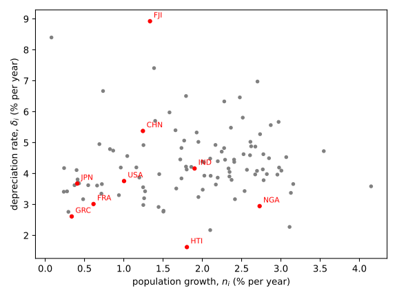
Country-specific convergence speeds
If we take the model seriously, the convergence speed of country \(i\) is \(\beta_i = (1-\alpha)(n_i+x+\delta_i)\), and the growth equation becomes
\begin{equation*} \bar g_{y,i} = x + \frac{1-e^{-\beta_i t}}{t}\left(a + \frac{\alpha}{1-\alpha}\bigl(\log s_i - \log(n_i+x+\delta_i)\bigr) - \log y_i(0)\right) + u_i \end{equation*}with \(u_i = \varepsilon_i(1-e^{-\beta_i t})/t\). The factor multiplying the bracket differs across countries and depends on \(\alpha\): the equation is no longer linear in the parameters, and OLS no longer applies. There are still only two parameters to estimate, \(\alpha\) and \(a\), since the speed of each country follows from \(\alpha\) and from its own \(n_i\) and \(\delta_i\). We do not need to estimate 110 convergence speeds.
Dividing the equation by \((1-e^{-\beta_i t})/t\) gives
\begin{equation*} \frac{t(\bar g_{y,i} - x)}{1-e^{-\beta_i t}} + \log y_i(0) = a + \frac{\alpha}{1-\alpha}\bigl(\log s_i - \log(n_i+x+\delta_i)\bigr) + \varepsilon_i \end{equation*}When \(\beta_i t\) is large, the left-hand side tends to \(\log y_i(t) - xt\): we recover the level regression of Mankiw, Romer and Weil, which explains income per head of a country assumed to be at its steady state. The growth equation also accounts for the distance still to be travelled. This way of writing the model is illuminating, but it does not provide a good estimator: the left-hand side depends on \(\alpha\), and minimising the sum of squares of its residuals overstates the convergence speed (see exercise 4).
Estimation
Non-linear least squares
Let \(\theta\) be the vector of parameters and \(f_i(\theta)\) the growth rate the model predicts for country \(i\). The non-linear least squares (NLS) estimator minimises, like the OLS estimator, the sum of squared residuals:
\begin{equation*} \hat\theta = \arg\min_{\theta}\;\mathrm{SSR}(\theta) = \sum_{i=1}^{N}\bigl(\bar g_{y,i} - f_i(\theta)\bigr)^2 \end{equation*}OLS is the special case in which \(f_i(\theta)\) is linear in \(\theta\). The first-order conditions, \(\sum_i \frac{\partial f_i}{\partial\theta}(\hat\theta)\bigl(\bar g_{y,i} - f_i(\hat\theta)\bigr) = 0\), now form a non-linear system with no explicit solution. It is solved by iteration. The Gauss-Newton algorithm replaces, at the point \(\theta_k\), the function \(f\) by its linear approximation \(f(\theta_k) + J_k(\theta - \theta_k)\), where \(J_k\) is the matrix of the derivatives \(\partial f_i/\partial\theta\) (the Jacobian), and then applies OLS:
\begin{equation*} \theta_{k+1} = \theta_k + (J_k'J_k)^{-1}J_k'\bigl(\bar g_y - f(\theta_k)\bigr) \end{equation*}
The Jacobian plays the role of the matrix of regressors: at convergence, the
variance of the estimator is estimated, as for OLS, by
\(\hat\sigma^2(J'J)^{-1}\), with \(\hat\sigma^2 = \mathrm{SSR}(\hat\theta)/N\).
We use the least_squares function of SciPy, which refines this algorithm,
and we run it from several starting points to make sure that the minimum we
find is the lowest one.
Maximum likelihood
The error term, \(u_i = \varepsilon_i w_i(\theta)\) with \(w_i(\theta) = (1-e^{-\beta_i t})/t\), does not have the same variance in every country. But we do not have to treat this heteroskedasticity as a nuisance of unknown form: the model produces it, and gives its exact form, \(\mathbb{V}(u_i) = \sigma^2w_i(\theta)^2\). We may as well use it. If the \(\varepsilon_i\) are normal and independent, the log-likelihood is, up to a constant,
\begin{equation*} \ell(\theta,\sigma^2) = -\frac{N}{2}\log\sigma^2 - \sum_{i=1}^{N}\log w_i(\theta) - \frac{1}{2\sigma^2}\sum_{i=1}^{N}\left(\frac{\bar g_{y,i} - f_i(\theta)}{w_i(\theta)}\right)^2 \end{equation*}Replacing \(\sigma^2\) by the estimator that maximises it, \(\hat\sigma^2(\theta) = \frac{1}{N}\sum_i\bigl((\bar g_{y,i} - f_i(\theta))/w_i(\theta)\bigr)^2\), gives the concentrated criterion
\begin{equation*} \ell(\theta) = -\frac{N}{2}\log\left(\frac{1}{N}\sum_{i=1}^{N}\left(\frac{\bar g_{y,i} - f_i(\theta)}{w_i(\theta)}\right)^2\right) - \sum_{i=1}^{N}\log w_i(\theta) \end{equation*}It has two terms. The first is the sum of squared residuals weighted by the inverse of their standard deviation: a country counts the more heavily the smaller its error is supposed to be. The second penalises values of \(\theta\) that inflate these standard deviations. Without it, weighting alone would attract the estimator towards high speeds, since dividing by large numbers would be enough to reduce the criterion (see exercise 4).
When the convergence speed is common, \(w_i\) no longer depends on \(i\) and the two terms cancel out exactly: the criterion reduces to \(-\frac{N}{2}\log\bigl(\mathrm{SSR}(\theta)/N\bigr)\), which the OLS estimator maximises. Maximum likelihood therefore departs from the OLS estimates of Mankiw, Romer and Weil only through what country-specific speeds add, and the five specifications can be compared by the same log-likelihood.
We maximise \(\ell\) numerically, with minimize of SciPy, starting from the
NLS estimate. The standard errors are the square roots of the diagonal of the
inverse Hessian of \(-\ell\), computed by finite differences. We compare them
with standard errors robust to heteroskedasticity, computed on the weighted
residuals: if the model is right about the form of the variance, the two
should be close. Restrictions are tested by a likelihood ratio,
\(2\bigl(\ell(\hat\theta) - \ell(\tilde\theta)\bigr)\), which follows a
\(\chi^2\) distribution with one degree of freedom under the hypothesis being
tested.
We compare four specifications. M0' and M1 have the same number of parameters; the last three are nested, each adding one restriction to the previous one:
- M0': the Mankiw, Romer and Weil regression, estimated by OLS with \(\log(n_i + x + \delta_i)\) instead of \(\log(n_i + 0.05)\) (and M0, the original regression, on the same sample);
- M1: the same equation, but with a country-specific speed, \(\beta_i = \theta(n_i+x+\delta_i)\), where \(\theta\) is a free parameter, and free coefficients on \(\log s_i\) and \(\log(n_i+x+\delta_i)\) in the bracket. Only the structure of the speeds changes relative to M0';
- M2: M1 with opposite coefficients on \(\log s_i\) and \(\log(n_i+x+\delta_i)\), equal to \(\pm\alpha/(1-\alpha)\), as in the Solow model;
- M3: M2 with \(\theta = 1-\alpha\), that is the full Solow model, in which the same elasticity \(\alpha\) pins down both the steady state and the convergence speed.
def growth(p, model, ly0):
    """Growth rate predicted by a specification, for the parameters p."""
    if model == 'M1':
        theta, a, a2, a3 = p
    elif model == 'M2':
        theta, a, alpha = p
        a2, a3 = alpha/(1 - alpha), -alpha/(1 - alpha)
    else:
        a, alpha = p
        theta, a2, a3 = 1 - alpha, alpha/(1 - alpha), -alpha/(1 - alpha)
    w = 1 - np.exp(-theta*c*t)
    return x + w/t*(a + a2*np.log(s) + a3*np.log(c) - ly0)

BOUNDS = {'M1': ([1e-4, -np.inf, -np.inf, -np.inf], [3, np.inf, np.inf, np.inf]),
          'M2': ([1e-4, -np.inf, 0.01], [3, np.inf, 0.99]),
          'M3': ([-np.inf, 0.01], [np.inf, 0.99])}

def nls(model, g, ly0, starts):
    """NLS estimator, the best of several starting points."""
    residuals = lambda p: g - growth(p, model, ly0)
    trials = [least_squares(residuals, p0, bounds=BOUNDS[model]) for p0 in starts]
    return min(trials, key=lambda e: e.cost), trials

def weights(p, model):
    """Relative standard deviation of the error of country i, w_i(theta)."""
    theta = p[0] if model != 'M3' else 1 - p[1]
    return (1 - np.exp(-theta*c*t))/t

def loglik(p, model, g, ly0):
    """Concentrated log-likelihood, up to a constant."""
    w = weights(p, model)
    u = (g - growth(p, model, ly0))/w
    return -N/2*np.log(u @ u/N) - np.sum(np.log(w))

def mle(model, g, ly0, start):
    """Maximum likelihood, starting from the NLS estimate."""
    bounds = [(max(lo, -50), min(hi, 50)) for lo, hi in zip(*BOUNDS[model])]
    return minimize(lambda p: -loglik(p, model, g, ly0), start,
                    method='L-BFGS-B', bounds=bounds)

def standard_errors(p, model, g, ly0, h=1e-4):
    """Standard errors of the MLE: from the Hessian, then robust ones as a check."""
    k = len(p)
    H = np.empty((k, k))
    for i in range(k):
        for j in range(k):
            ei, ej = np.zeros(k), np.zeros(k)
            ei[i], ej[j] = h, h
            H[i, j] = -(loglik(p + ei + ej, model, g, ly0)
                        - loglik(p + ei - ej, model, g, ly0)
                        - loglik(p - ei + ej, model, g, ly0)
                        + loglik(p - ei - ej, model, g, ly0))/(4*h*h)
    w = weights(p, model)
    f = least_squares(lambda q: (g - growth(q, model, ly0))/w, p, bounds=BOUNDS[model])
    J, e = f.jac, f.fun
    A = np.linalg.inv(J.T @ J)
    return np.sqrt(np.diag(np.linalg.inv(H))), np.sqrt(np.diag(A @ (J.T*e**2) @ J @ A))
Results
logliks = {}
for name, z in (('M0', np.log(n + 0.05)), ("M0'", np.log(c))):
    X = np.column_stack([np.ones(N), ly0, np.log(s), z])
    b, V, ssr = ols(X, g)
    logliks[name] = -N/2*np.log(ssr/N)
    print(name, b.round(4), (b/np.sqrt(np.diag(V))).round(2), speed(b[1]),
          b[2]/(b[2] - b[1]), R @ b/np.sqrt(R @ V @ R), ssr, logliks[name])

STARTS = {'M1': [[th, 8, 2, -2] for th in (0.05, 0.1, 0.3)],
          'M2': [[th, 7, al] for th in (0.05, 0.1, 0.3) for al in (0.4, 0.7)],
          'M3': [[7, al] for al in (0.3, 0.5, 0.7)]}
estimates = {}
for name in ('M1', 'M2', 'M3'):
    start, trials = nls(name, g, ly0, STARTS[name])
    fit = mle(name, g, ly0, start.x)
    estimates[name], logliks[name] = fit.x, -fit.fun
    classical, robust = standard_errors(fit.x, name, g, ly0)
    print(name, start.x.round(4), fit.x.round(4), classical.round(4),
          robust.round(4), logliks[name], sorted({round(2*e.cost, 6) for e in trials}))
NLS, which provides the starting point, reaches the same minimum whatever the starting value, and the maximisation of the likelihood then starts from its solution. The table below summarises the estimates, with the standard errors from the Hessian in brackets; the robust standard errors differ little (0.042 instead of 0.049 for the \(\alpha\) of M2), which suggests that the form of the variance given by the model is not contradicted by the data. For M0 and M0', the speed is common to all countries and \(\alpha\) follows from the coefficients, \(\alpha = a_2/(a_2 - a_1)\) (see exercise 1); for M1, M2 and M3, the reported speed is the median of the \(\beta_i\).
| Model | Speed (% per year) | \(\alpha\) | \(\theta\) | \(\ell\) |
|---|---|---|---|---|
| M0 | 1.43 | 0.581 | 480.22 | |
| M0' | 0.76 | 0.745 | 466.46 | |
| M1 | 0.77 | 0.094 (0.037) | 467.75 | |
| M2 | 0.84 | 0.710 (0.049) | 0.102 (0.037) | 467.40 |
| M3 | 2.85 | 0.653 (0.030) | \(1-\alpha\) | 460.28 |
def lr_test(restricted, free):
    LR = 2*(logliks[free] - logliks[restricted])
    return LR, 1 - stats.chi2.cdf(LR, 1)

print(lr_test('M2', 'M1'), lr_test('M3', 'M2'))
theta = {'M1': estimates['M1'][0], 'M2': estimates['M2'][0],
         'M3': 1 - estimates['M3'][1]}
for name, th in theta.items():
    beta = th*c
    print(name, np.median(beta), beta.min(), codes[beta.argmin()],
          beta.max(), codes[beta.argmax()], np.log(2)/np.median(beta))
Three results stand out.
Replacing the common 0.05 by country-specific rates worsens the fit. The log-likelihood goes from 480.2 (M0) to 466.5 (M0'), and the coefficient on \(\log(n_i + x + \delta_i)\) is no longer significant (its \(t\) statistic is \(-0.76\)). The restriction \(a_2 + a_3 = 0\) is no longer rejected (\(1.06\)), but mostly because this regressor no longer explains much. In M0, \(\log(n_i + 0.05)\) varies only with population growth, which is negatively correlated with the growth of income per head (the correlation coefficient is \(-0.38\)). In M0', its variation comes mostly from depreciation, which is on the contrary positively correlated with growth (\(0.22\)), so that \(\log(n_i + x + \delta_i)\) is barely correlated with growth at all (\(-0.06\)). The model nevertheless predicts that faster depreciation lowers long-run income, and hence growth. The PWT depreciation rate is an average of asset-specific rates, weighted by the composition of capital: it reflects the structure of investment as much as the wear and tear of capital.
Country-specific speeds barely fit better than a common speed. With the same regressors, M1 and M0' have the same number of parameters and close log-likelihoods (467.75 against 466.46). The data hardly distinguish between the two structures. The interest of country-specific speeds lies in their consistency with the model, and in the test they allow: in M2 the parameter \(\theta\) that governs the speed is estimated independently of \(\alpha\), and the Solow model imposes \(\theta = 1 - \alpha\). The restriction of M2 on the coefficients in the bracket is not rejected (likelihood ratio of 0.71, p-value of 0.40).
The full Solow model is rejected. The restriction \(\theta = 1-\alpha\) costs 7.1 points of log-likelihood, that is a likelihood ratio of \(14.2\) and a p-value of 0.00016. Without the restriction, the median speed is 0.84% per year, a half-life of 82 years, and \(\alpha\) is estimated at 0.71. With the restriction, the median speed is 2.9% per year (a half-life of 24 years), and ranges from 1.7% in Greece to 4.3% in Fiji. The figure below shows the log-likelihood of M2 as a function of \(\alpha\) and \(\theta\) (the constant \(a\) is optimised for each pair). The maximum is far from the line \(\theta = 1-\alpha\): the value of \(\alpha\) that accounts for income differences across countries implies far too fast a convergence.
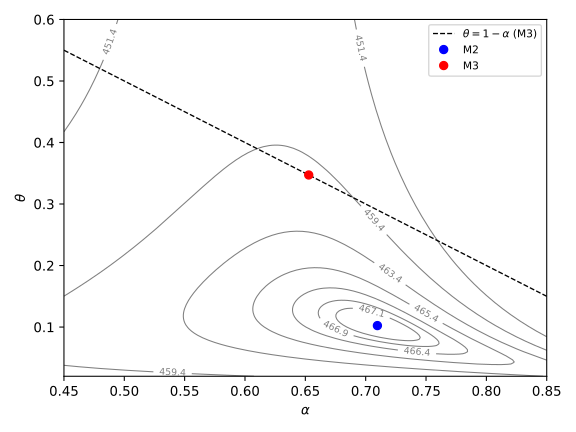
This is, in another guise, the finding that leads Mankiw, Romer and Weil to the model augmented with human capital: the convergence speed becomes \(\beta_i = (1-\alpha-\lambda)(n_i+x+\delta_i)\), where \(\lambda\) is the elasticity of output with respect to human capital, and a larger share for capital broadly defined slows convergence down.
Endogeneity
All these estimates assume that the disturbance \(\varepsilon_i\) is correlated neither with the saving and population growth rates, nor with initial income. The course states the second assumption explicitly, \(\mathrm{Cov}(\varepsilon_i, \log y_j(0)) = 0\). It is nevertheless hard to defend: since \(\log y_i(0) = a + \varepsilon_i + \log\hat y_i(0)\), a country whose labour efficiency is high has, other things being equal, a high initial income. In the growth equation, initial income is then correlated with the error term, which contains \(\varepsilon_i\), and the estimators no longer converge to the true values of the parameters.
To measure the effect of this correlation, let us simulate data from model M3, keeping the estimated values of \(\alpha\) and \(a\), the observed saving, population growth and depreciation rates, and a standard deviation of \(\varepsilon_i\) taken from the residuals. Incomes in 2023 are computed with the exact solution of the Solow equation, not with its log-linear approximation: writing \(z = \hat k^{1-\alpha}\), \(z(t) = z^{\star} + (z(0) - z^{\star})e^{-\beta_i t}\), where \(z^{\star} = s_i/(n_i+x+\delta_i)\) (see the note on simulating the Solow model). We consider two cases:
- in the first, initial income is the observed one, and it is initial output per efficiency unit of labour, \(\log\hat y_i(0)\), that adjusts to \(\varepsilon_i\): the assumption of the course holds;
- in the second, \(\log\hat y_i(0)\) is fixed, and initial income contains \(\varepsilon_i\).
In each case we simulate 500 samples, estimate M2 and M3 by maximum likelihood, and test \(\theta = 1-\alpha\) at the 5% level.
a3, alpha3 = estimates['M3']
beta3 = (1 - alpha3)*c
epsilon = (g - growth(estimates['M3'], 'M3', ly0))/weights(estimates['M3'], 'M3')
sigma = epsilon.std()
rng = np.random.default_rng(2014)

def simulation(endogenous):
    """Simulated growth rates, from the exact solution, and initial incomes."""
    e = rng.normal(0, sigma, N)
    if endogenous:
        lyh0 = ly0 - a3
        ly0_sim = lyh0 + a3 + e
    else:
        ly0_sim = ly0
        lyh0 = ly0 - a3 - e
    z0 = np.exp(lyh0*(1 - alpha3)/alpha3)
    z = s/c + (z0 - s/c)*np.exp(-beta3*t)
    lyt = a3 + e + x*t + alpha3/(1 - alpha3)*np.log(z)
    return (lyt - ly0_sim)/t, ly0_sim

simulations = {}
for endogenous in (False, True):
    theta2, alpha3_sim, rejections = [], [], 0
    for r in range(500):
        g_sim, ly0_sim = simulation(endogenous)
        m2 = mle('M2', g_sim, ly0_sim, [0.1, 7, 0.6])
        m3 = mle('M3', g_sim, ly0_sim, [7, 0.6])
        LR = 2*(m3.fun - m2.fun)
        rejections += LR > stats.chi2.ppf(0.95, 1)
        theta2.append(m2.x[0])
        alpha3_sim.append(m3.x[1])
    simulations[endogenous] = np.array(theta2)
    print(endogenous, np.mean(alpha3_sim), np.median(theta2), rejections/500)
print(sigma, 1 - alpha3, simulations[False].min(), np.percentile(simulations[False], 5),
      simulations[True].max(), np.percentile(simulations[True], 95))
In the first case, the estimator of \(\alpha\) in M3 is almost unbiased (0.655 on average for a true value of 0.653): the log-linear approximation is not the problem. The test rejects the restriction \(\theta = 1-\alpha\) in 8% of the samples, somewhat more than the 5% announced: with 110 countries, the approximation of the distribution of the likelihood ratio by a \(\chi^2\) remains crude. In the second case, the estimate of \(\alpha\) rises to 0.74, the median of \(\hat\theta\) falls to 0.06 whereas the true value is 0.35, and the test rejects the restriction in every sample. The figure below compares the two distributions of \(\hat\theta\) with the estimate obtained on the data.
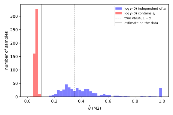
The estimate obtained on the data, 0.102, is below every estimate of the first case, the smallest of which is 0.17, and above every estimate of the second, the largest of which is 0.09. It could come from a Solow model in which initial income contains only part of \(\varepsilon_i\): the rejection of the full model would then come from that correlation, and not from a failure of the model. It could also come from a model in which the convergence speed is not the one of the Solow model: in a cross-section, we cannot tell. Nor can we instrument initial income by older incomes, which contain the same permanent component \(\varepsilon_i\). The second source of endogeneity, the correlation of \(\varepsilon_i\) with the saving and population growth rates, which Mankiw, Romer and Weil rule out by assumption, raises the same problem.
The usual answer is to follow countries over several periods. Splitting 1960-2023 into periods of length \(\tau\), the growth equation reads
\begin{equation*} \log y_{i,k+1} = \rho_i\log y_{i,k} + (1-\rho_i)\frac{\alpha}{1-\alpha}\bigl(\log s_{i,k} - \log(n_i+x+\delta_i)\bigr) + \mu_i + \gamma_{i,k} + v_{i,k+1} \end{equation*}with \(\rho_i = e^{-\beta_i\tau}\), a country effect \(\mu_i = (1-\rho_i)\log A_i(0)\), which absorbs \(\varepsilon_i\), and a trend term \(\gamma_{i,k}\) known up to \(\alpha\). This fixed effect can be removed by differencing the equation, and incomes of earlier periods then become valid instruments. The literature shows, however, that the answer depends a great deal on the method. With fixed effects, Islam (1995) finds speeds of 4 to 5% per year on the large samples, and above 9% for the OECD countries. With the generalised method of moments (GMM) applied to the equation in differences, Caselli, Esquivel and Lefort (1996) find about 10%. Bond, Hoeffler and Temple (2001) show that the instruments are then weak, and find 2 to 4% with the system GMM estimator. The simulations of Hauk and Wacziarg (2009) indicate that fixed effects and difference GMM greatly overstate the convergence speed, and that the cross-section estimator, the one used in this note, is the least biased in the presence of measurement error. Finally, when each country has its own speed, unrelated to the model, Lee, Pesaran and Smith (1997) find average speeds of the order of 30% per year, very imprecisely estimated. The structure \(\beta_i = (1-\alpha)(n_i+x+\delta_i)\) lies between these two extremes: it allows speeds to differ, but ties them to a single parameter. Estimating it on a panel is the subject of the next note.
Conclusion
Taking the convergence speed of the Solow model seriously only requires a change of estimator: a common capital share is enough to give each country its own speed, and the model also says how countries should be weighted, which maximum likelihood exploits. On the PWT data, these country-specific speeds barely fit better than a common speed, and the full Solow model is rejected, because the capital share that accounts for income differences implies too fast a convergence. This verdict is fragile, however: the same estimation, applied to data simulated from an exact Solow model, leads to the same rejection as soon as initial income contains labour efficiency. Only a panel estimation can separate the two explanations.
Exercises
Assume the convergence speed is common to all countries. Express the coefficients \(a_1\) and \(a_2\) of the Mankiw, Romer and Weil regression as functions of \(\alpha\), \(\beta\) and \(t\), and show that \(\alpha = a_2/(a_2 - a_1)\). Compute the value of \(\alpha\) implied by the estimates of M0 and M0', and compare it with that of M2.
Solution
In the growth equation, initial income is multiplied by \(a_1 = -(1-e^{-\beta t})/t\) and the logarithm of the saving rate by \(a_2 = \frac{1-e^{-\beta t}}{t}\frac{\alpha}{1-\alpha} = -a_1\frac{\alpha}{1-\alpha}\). Hence \(\alpha/(1-\alpha) = -a_2/a_1\), that is \(\alpha = a_2/(a_2 - a_1)\). The estimates of M0 give \(\hat a_1 = -0.0094\) and \(\hat a_2 = 0.0131\), hence \(\alpha = 0.58\); those of M0', \(\hat a_1 = -0.0061\) and \(\hat a_2 = 0.0177\), hence \(\alpha = 0.75\). The value of M2, 0.71, lies between the two. In all three cases the capital share is well above the value of \(1/3\) that is usually retained. And even with these high values, the convergence speed implied by the model, \((1-\alpha)(n_i+x+\delta_i)\), exceeds the estimated speed in every country.
Compute the half-life of the gap to the steady state, \(\log 2/\beta_i\), for the country that converges most slowly and for the one that converges fastest, with the estimates of M2 and M3.
Solution
for name in ('M2', 'M3'):
    beta = theta[name]*c
    print(name, codes[beta.argmin()], np.log(2)/beta.min(),
          codes[beta.argmax()], np.log(2)/beta.max())
The speed is lowest in Greece, where population grows slowly and capital depreciates slowly, and highest in Fiji, where depreciation is the fastest in the sample. With M2, the half-life ranges from 55 years in Fiji to 137 years in Greece; with M3, from 16 to 40 years. Country-specific speeds are not a detail: from one country to another, the half-life varies by a factor of more than two.
Program the Gauss-Newton algorithm to estimate M3, computing the Jacobian by
finite differences, and check that it converges to the estimate obtained with
least_squares.
Solution
def gauss_newton(p, iterations=8, h=1e-6):
    for k in range(iterations):
        e = g - growth(p, 'M3', ly0)
        J = np.column_stack([(growth(p + h*u, 'M3', ly0)
                              - growth(p - h*u, 'M3', ly0))/(2*h)
                             for u in np.eye(len(p))])
        p = p + np.linalg.solve(J.T @ J, J.T @ e)
        print(k, p.round(6), e @ e)
    return p

gauss_newton(np.array([7.0, 0.5]))
print(estimates['M3'].round(6))
Starting from \(a = 7\) and \(\alpha = 0.5\), the algorithm reaches in a few
iterations the estimate of least_squares, \(\hat a = 6.570\) and
\(\hat\alpha = 0.645\), and the sum of squared residuals stops falling. Each
iteration is an OLS regression of the residuals on the columns of the
Jacobian. It is from this point that the maximisation of the likelihood
starts, and it then moves the estimate to \(\hat\alpha = 0.653\).
Write \(w_i(\theta) = (1-e^{-\beta_i t})/t\), so that \(\bar g_{y,i} - f_i(\theta) = w_i(\theta)\varepsilon_i\). A colleague suggests estimating \(\theta\) by minimising \(\sum_i\bigl((\bar g_{y,i} - f_i(\theta))/w_i(\theta)\bigr)^2\), in order to get rid of the heteroskedasticity. Why does this estimator tend to overstate the convergence speed?
Solution
The weights \(1/w_i(\theta)\) depend on the parameters. And \(w_i\) increases with the convergence speed: for given residuals, raising the speed reduces the criterion, simply because one divides by a larger number. The estimator is therefore attracted towards high speeds, irrespective of the fit. This is exactly what the term \(-\sum_i\log w_i(\theta)\) of the log-likelihood prevents. This is what we observe on our data:
def divided_nls(model, p0):
    def residuals(p):
        th = p[0] if model == 'M2' else 1 - p[1]
        return (g - growth(p, model, ly0))*t/(1 - np.exp(-th*c*t))
    return least_squares(residuals, p0, bounds=BOUNDS[model]).x

p2, p3 = divided_nls('M2', [0.1, 7, 0.6]), divided_nls('M3', [7, 0.6])
print(p2, np.median(p2[0]*c), p3, np.median((1 - p3[1])*c))
With M3, the median speed goes from 2.9% to 3.7% per year. With M2, where the speed does not depend on \(\alpha\), \(\theta\) reaches the upper bound imposed on the optimisation, \(\theta = 3\), that is a median speed of 25% per year. When the variance of an error depends on the parameters, weighting alone is therefore not enough. One can either fix the weights, computing them from a first estimation and then holding them constant, or maximise the likelihood, which penalises high speeds through the term \(-\sum_i\log w_i(\theta)\). On our data, the two solutions give close estimates.
References
The conditional convergence regression is due to Mankiw, N. G., Romer, D. and Weil, D. (1992), "A Contribution to the Empirics of Economic Growth", Quarterly Journal of Economics, 107(2), 407-437. The panel estimates cited above are those of Islam, N. (1995), "Growth Empirics: A Panel Data Approach", Quarterly Journal of Economics, 110(4), 1127-1170, of Caselli, F., Esquivel, G. and Lefort, F. (1996), "Reopening the Convergence Debate: A New Look at Cross-Country Growth Empirics", Journal of Economic Growth, 1(3), 363-389, of Bond, S., Hoeffler, A. and Temple, J. (2001), "GMM Estimation of Empirical Growth Models", CEPR Discussion Paper 3048, and of Lee, K., Pesaran, M. H. and Smith, R. (1997), "Growth and Convergence in a Multi-Country Empirical Stochastic Solow Model", Journal of Applied Econometrics, 12(4), 357-392. The simulations are those of Hauk, W. and Wacziarg, R. (2009), "A Monte Carlo Study of Growth Regressions", Journal of Economic Growth, 14(2), 103-147. For an overview, see Durlauf, S., Johnson, P. and Temple, J. (2005), "Growth Econometrics", in Aghion, P. and Durlauf, S. (eds), Handbook of Economic Growth, vol. 1A, chapter 8, 555-677.
The data come from version 11.0 of the Penn World Tables (Groningen Growth and Development Centre, 2025, doi:10.34894/FABVLR), described in Feenstra, R., Inklaar, R. and Timmer, M. (2015), "The Next Generation of the Penn World Table", American Economic Review, 105(10), 3150-3182. On the Solow model itself, see the notes on the Solow model and on its simulation.